Devoured - October 09, 2026
OpenAI and Google have launched new agentic interfaces—Intelligent UI for ChatGPT and a universal Gemini agent—signaling a major industry shift toward interactive, multi-step autonomous workflows. Meanwhile, critical infrastructure projects like the DNS root key rollover and the CNCF’s AI-assisted graduation process highlight the growing role of AI in maintaining the reliability of foundational tech and open-source ecosystems.

Gemini Agent
Google launched a universal Gemini agent that supports multi-step orchestration, persistent memory, and model routing to manage autonomous workflows.
Deep dive
- Unified Agent: A single interface for querying, coding, and media creation.
- Persistence: Cloud-based memory ensures agents retain context across sessions and devices.
- Orchestration: Dynamically creates sub-agents to parallelize complex tasks.
- Model Choice: Flexible routing between Gemini, Anthropic Claude, and other models to optimize for cost and accuracy.
- Governance: Introduces Agent Gateway, a firewall for AI agents to enforce policy and security.
Decoder
- Knowledge Catalog: A centralized metadata repository for mapping business definitions across diverse data sources like SAP or Databricks.
- Borderless Lakehouse: An architecture allowing queries across AWS (S3), Azure, and Google Cloud without data movement or variable egress fees.
- Agent Gateway: A network-level security service that intercepts and validates agent traffic against organizational policies.
Original article
Full article content is not available for inline reading.
Security Swarm
Devin's new Security Swarm uses 'Agentic MapReduce' to parallelize vulnerability scanning and remediation across large codebases.
Deep dive
- Agentic MapReduce: A technique where a large repository is split into smaller chunks, processed independently by parallel agents, and then aggregated for a global view.
- Threat Model Generation: The tool automatically drafts a security profile defining sensitive assets, trust boundaries, and entry points.
- Sandbox Validation: The agent attempts to reproduce detected vulnerabilities by building and exercising the application in an isolated environment.
- Incremental Scanning: Auto Scan feature that only analyzes new commits since the last run, keeping compute costs bounded.
- Remediation: The system can open pull requests with suggested fixes, including automated regression tests.
- Ingestion: Supports importing results from existing tools like Semgrep or GitHub code scanning for unified triage.
Decoder
- RCE (Remote Code Execution): A vulnerability that allows an attacker to execute arbitrary commands on a target server.
- SSRF (Server-Side Request Forgery): A vulnerability where an attacker tricks a web application into making requests to an unintended location, such as internal services.
- MapReduce: A programming model for processing large data sets in parallel across a distributed system.
Original article
Security Swarm is Devin’s security scanning and remediation product. It builds a threat model tailored to your code, investigates and validates potential vulnerabilities, and helps you fix findings through pull requests. It can identify vulnerabilities like remote code execution (RCE), SQL injection, path traversal, server-side request forgery (SSRF), authorization bypasses, memory-safety bugs, denial-of-service vulnerabilities, and more. It can even identify chained exploits spanning multiple files. Security Swarm is a custom orchestration of Devins we are calling Agentic MapReduce. It divides your repo among parallel Devins, providing broad coverage and deep investigation while bounding cost, making it cost-effective to scan large codebases.
Prerequisites
To run a scan:
- Your organization must have access to the repository you want to scan.
- You need to be authorized to use Devin sessions.
- You need the Use code scans permission.
- To configure an Auto Scan schedule, you also need Manage code scans and permission to manage automations.
Run your first scan
- Open Security in the left sidebar and click Start scan.
- Under Single repo, choose a repository to scan.
- Optionally select a scan profile and a scan effort. Leaving the profile blank uses Security Swarm’s built-in security scan.
- Make sure Interactive mode is enabled.
- Click Run Scan.
- When the proposed threat model is ready, review it and either click Looks good, start scanning or provide feedback.
- As findings appear, review the evidence and act on the findings that need attention.
Review and act on findings
Open a scan to see its findings. The page displays a list of findings on the left, grouped by severity, and the selected finding’s details on the right. The status tabs show a live count:
- Open — needs attention.
- Reviewed — has been reviewed and no longer requires action.
- Dismissed — was determined as a false positive or duplicate.
What’s in a finding
A finding includes:
- Severity, status, exploitability, confidence, and category.
- The affected file path and code snippets.
- A description of the issue and a remediation recommendation.
- A sandbox validation result, supporting evidence, and validation artifacts.
- Associated pull requests and their open, merged, or closed state.
- Code owners and notes, when available.
Act on a finding
- Assign to Devin: Starts a Devin session to remediate the issue and open a pull request.
- Feedback: Sends context to a feedback session that refines the scan profile for future scans.
- Adjust: Overrides the finding’s severity, with optional context for Devin.
- Status menu: Marks the finding as Open, Reviewed, or Dismissed.
Scan profiles
A scan profile controls the scan’s scope and provides guidance for each stage of the scan. Every scan can use one profile.
Create a profile
- Generate with Devin — describe the application, threats, scope, exclusions, and severity standards in natural language.
- Create manually — fill in each profile input yourself.
Threat model
Assume an unauthenticated internet attacker or an authenticated user in one tenant.
Focus on public HTTP handlers, OAuth callbacks, API tokens, administrative actions,
and accesses to tenant-owned data. Treat internal development scripts and local-only
tools as out of scope. Prioritize authentication bypasses, cross-tenant access, token
leakage, injection, and SSRF.
Investigation guidance
Trace untrusted input from the route through middleware and service layers to the
sensitive operation. Check authentication, authorization, tenant scoping, validation,
and escaping at every boundary. Identify the exact reachable path and cite the relevant
files and lines. Do not report a theoretical issue when an effective mitigation blocks
the path.
Triage guidance
Group findings that share the same root cause. Treat unauthenticated remote code
execution and cross-tenant write access as critical. Treat cross-tenant read access and
credential disclosure as high. Treat single-user availability issues as medium unless
they can affect shared infrastructure. Label defense-in-depth recommendations as low.
Sandbox validation
Use the repository's documented development setup. Start the API and create two
non-production tenants with one test user in each. Attempt the suspected request as a
user from the other tenant, then verify both the HTTP response and persisted data.
Do not call production services or modify production data.
Remediation guidance
Prefer the smallest safe change and preserve existing public API behavior. Add a
regression test that fails before the fix and passes afterward. Run the affected package's
lint and test commands. Avoid major dependency upgrades unless the vulnerability cannot
be fixed safely without one.
Scale scanning
| Mode | What it does |
|---|---|
| Single repo | One scan of one repository. |
| Multi-repo | One scan across up to 200 repositories. |
| Bulk scan | A separate, independent scan for every matching repository. |
| Ingest findings | Imports findings from your existing tooling or reports. |
Access and permissions
| Permission | What it unlocks |
|---|---|
| View code scans | View scans, profiles, findings, and associated scan sessions. |
| Use code scans | Start scans, create organization profiles, submit finding feedback, adjust findings, change finding statuses, and assign findings to Devin. |
| Manage code scans | Archive or unarchive scans and configure Auto Scan schedules. |
| Manage account code scans | Promote organization profiles to enterprise scope and edit or archive enterprise profiles. |
FAQ
How does Security Swarm reduce false positives?
Security Swarm investigates potential vulnerabilities in the context of your repository rather than reporting risky patterns in isolation. Devin traces relevant data flows, checks for validation and authorization controls, and evaluates whether the issue has a concrete security impact.
What does sandbox validation add?
Sandbox validation attempts to reproduce a finding by building and exercising the application in an isolated environment. A successful validation provides stronger evidence of exploitability.
How does Security Swarm find vulnerabilities that span multiple files?
Security Swarm analyzes parts of the repository in parallel and combines the results into a repository-wide view. This allows it to identify relationships between components.
Amazon builds 1,000th satellite, will launch space internet service by end of year
Amazon’s Project Kuiper is weeks away from launching commercial broadband service, entering a market dominated by SpaceX's Starlink.
Deep dive
- Manufacturing Scalability: Amazon transitioned from taking six months to build 27 satellites to building 27 per week.
- Performance: Amazon claims 1 Gbps downlink and 400 Mbps uplink, targeting 3x downlink and 8-10x uplink speeds compared to Starlink.
- Security: Offers AES-256 encryption and private network gateways that bypass the public internet directly into data centers.
- Integration: Consumers can expect integration with existing Amazon services like Prime, eero, and Ring.
- Launch Strategy: Amazon utilizes a multi-vendor approach with ULA, Blue Origin, and Arianespace to mitigate launch risks.
Decoder
- Leo (Low-Earth orbit): Satellites orbiting between 160 and 2,000 km, used for high-speed internet because their proximity allows for lower latency compared to geostationary satellites.
Original article
The world’s largest retailer wants to sell you something else—Internet from space.
Amazon has been developing a constellation of satellites to deliver broadband Internet from low-Earth orbit for the better part of a decade, and the company is just about ready to pull back the curtain. It is entering a market that SpaceX, with its Starlink Internet, has dominated for the last half-decade. Amazon’s debut into satellite Internet is being closely watched, not just by some consumers, but by businesses ranging from airlines to shipping companies to governments. Broadband Internet from orbit has proven broadly useful for a lot of purposes, from video games to commerce to warfighting.
But until now, most people had to buy it from Elon Musk and SpaceX. OneWeb has only offered limited services, leaving Amazon as the only real competitor to deliver high-speed Internet globally. Moreover, at the head of the company’s broadband efforts is Rajeev Badyal, who led Starlink during its early years, but whom Musk fired eight years ago for moving too cautiously on Starlink.
In a wide-ranging interview this week with Badyal and two other senior Amazon officials developing the constellation—Paul Palcisco, director of production; and Chris Weber, vice president of business—Ars was able to learn that the Amazon Leo project is nearing several critical milestones. At its Kirkland, Washington-based factory, the company recently manufactured its 1,000th satellite, will soon make its debut on the Vulcan rocket, and is just weeks away from offering commercial service for the first time.
We discussed the challenges that Amazon had to overcome to become the world’s second-largest satellite manufacturer (behind SpaceX), and reach the point where it can build a handful of satellites every day. Badyal also confirmed that the Vulcan rocket’s upcoming return-to-flight mission will carry Amazon Leo satellites and that another Vulcan rocket standing right next to it is also being prepared to launch this year with more Amazon satellites.
And finally, and perhaps most consequentially, Amazon is close to offering its service commercially. The company has been busy signing contracts—Delta Airlines’ agreement to use Amazon over Starlink on its planes has upset SpaceX founder Elon Musk, to put it mildly—and consumers are about to get an alternative to the industry-leading space broadband service. Are Amazon and its founder, Jeff Bezos, ready to compete?
The following interview has been lightly edited for clarity.
Ars: How did you overcome production hell to reach a point where you’re building satellites at scale?
Rajeev Badyal: Building a couple of satellites is pretty straightforward, but building at scale is just exponentially harder. Our job one was to design a satellite that is mass-producible. So you have to take manufacturing into account from day one. But in the real world it never turns out that way, because design engineers, the first thing they want to do is solve for making sure it works. Then they think about manufacturability as the next step. But we pushed really hard for a culture where we could do both, get a design that works and it’s manufacturable. Even in doing so, when you actually get to the real product, and you put it through its paces, you find a lot of gaps. You find gaps in quality. You find gaps in reliability. You find issues with parts.
You have to work on every single detail of what needs to be done. I mean, it was brutal. Teams worked hand-in-hand to continuously improve processes, to continuously improve designs, to continuously improve our training. Imagine when you open a factory and you introduce people to a brand-new design, a set of technicians who are coming online, who are skilled but are not skilled in satellites. How you train them, how you bring them up to speed, how you find defects in real time. There’s a massive amount of work that went into this. I would say the team, the manufacturing operations and the dev teams together, did unbelievably fantastic work last year. It took us six months to make our first 27 satellites. Now we can easily make 27 a week. That’s how far we have come. But it is relentless focus on engineering, improving processes, and just getting better and better at what we do. It just takes an enormous amount of effort to get that done.
Ars: How did you go about setting up the factory?
Paul Palcisco: We built the factory as we were designing the satellites. So we didn’t have a product yet. We had to work closely with our engineering partners to understand what they were designing, so that we knew what those processes needed to look like. And so we took an empty 170,000-square-foot building in December 2022, and we turned it over the next 15 months into a satellite factory, and we built the first qualification satellite there, right? And we learned so much through that process of what we needed to fix. Because I’ll tell you, as soon as we opened the doors in that factory, we needed to change it.
Ars: How much of your satellite manufacturing is vertically integrated?
Palcisco: We looked very carefully at vertical integration, where it makes the most sense for us. There’s certain components where there are external sources that have decades of experience doing those parts, and it didn’t make sense for us to try to replicate all of that experience. Where we focus internally is where we add the most value, which essentially is ‘what are our highest value IP products?’ We want to keep those in-house because nobody else is building those, and then we work up from there in terms of building and testing the final products in our factory.
Ars: Can you give me an example of a high IP product or component?
Palcisco: A great example is our propulsion system, right? Our propulsion system is designed and built entirely in-house.
Ars: Over the last several years, as you’re scaling up production, what has been the biggest surprise or the biggest technical challenge that you’ve had to overcome?
Palcisco: I think our biggest technical challenge has been testing. If you go back to traditional space testing, it’s extremely rigorous. It falls back into a lot of NASA standards that were written several decades ago. SMC-S-016 is a great example of that, and that’s where we started, right? Because we wanted to have the highest-quality product. But then the challenge comes back to scale. Those testing procedures take days and weeks, and so what we’ve done over the last two years is blend those testing procedures with higher-volume testing procedures out of things like consumer electronics, where we can actually maintain or even increase the strength of screen of that test, so it’s a more robust test. But now we do it in much shorter amounts of time. So the testing that used to take us days and weeks we can now do in hours and ensure the same quality, so that when a satellite leaves our factory we know it’s good.
Ars: How long does it take to manufacture a satellite, starting at the first station in the factory, to getting through testing and packing it for shipping?
Palcisco: It’s on the order of magnitude of several weeks. I’ll say this, as we learn and as we incorporate changes into a satellite, we can do that within one to two weeks. We actually now pace the factory based on the modeling of our launch cadence, and how much of a finished goods buffer we want in front of that launch cadence. Our real mission is to make sure we never have a rocket where we don’t already have satellites ready for it. So as our launch partners increase their cadences, we want to be able to respond immediately with satellites that are already ready to go for them.
Ars: I want to get to launch in a moment. But first, Rajeev, this is a crazy industry in that there’s so much capital needed up front, and all this production and technical work before you get any data back from space. I guess you have to start with a lot of faith that this is all going to work out in the end?
Badyal: It’s faith in having a team around you that is world-class. When you have a team around you like we do, you have a lot of confidence that hey, we can solve it. We started off with a clean sheet of paper and came up with this design constellation. We sized everything in the first three months, like capacity, capability. We set our architecture within the first three months. Then we started developing all the hardware. As you do these things, the biggest concern you always have is, hey, is this architecture going to work? And is it going to be able to deliver the performance, the capacity, and the capability that you, that we, envisioned back in 2018?
It wasn’t till early this year that you could confirm that all the decisions that we made in our silicon design, in our antenna design, in our customer terminal design, in our gateway design, they will all come together and meet the performance needs. Right now, I’m actually watching Formula One on my phone. This is Leo running on my phone, and the antennas on the rooftop of this building, and the indoor unit is right behind the wall where I’m sitting. So it’s a demonstration of how well the network is already working today, and it meets all the performance requirements. But that took a long time to get to this point. And there are times when you doubt yourself. And that moment is pretty special when it does work.
Ars: Paul mentioned the launch market and not wanting to have rockets waiting around for satellites. Obviously, it seems like it’s a little bit the other way around. Can one of you talk about the challenges you’ve faced in the launch industry, and a little bit about the frustration you’ve experienced as a result of that?
Badyal: From day one we decided to go with a diverse set of partners to supply us with rockets. We started off with ULA, Blue Origin, Arianespace, and SpaceX. We signed deals with all four of them. We knew there was risk, but we had to get heavy lift vehicles. Because we had the diversity available to us, we are where we are today. Without that kind of plan, we probably would be in a far worse situation. Despite the delays Vulcan has had, despite the delays Blue Origin has had due to anomalies, there is no partner that isn’t working around the clock right now as we speak to get us launched as quickly as possible. It can be frustrating at times because things move, but at the same time, if this was easy, everybody else would be doing it, as you know.
Ars: It looks like Vulcan is coming back online soon.
Badyal: I can say we’re weeks away from launching on Vulcan. Things are on track. We’ll follow that with an Arianespace launch and at least one more Vulcan this year. I can also tell you, the infrastructure that we put and built with ULA now allows us to process two rockets simultaneously. So right now, there are two vehicle integration facilities, and both have a Vulcan rocket that is vertical and getting ready for our missions. So lots of progress there. I think once we get through this nozzle issue with Vulcan, which has been fixed, we expect a much more regular cadence with Vulcan. From time to time it can be frustrating, but I will say we see significant progress from everyone.
Ars: You have about 400 satellites in orbit now. Is that enough to launch your initial service to customers?
Badyal: We have enough already. And the next set of flights, they’re just additive to expanding our coverage, and adding more resiliency to the network as time goes on.
Ars: Can you talk about sort of your plans to roll out service? I know you talked about doing so before the end of the year, and it’s already early October.
Chris Weber: We have 396 satellites in orbit. We’re still doing work to raise them into final position, and then you know there’s a lot of work on the ground to do. But the plan is to launch initial service in 2026.
Ars: What do you see as your competitive advantage with Starlink? How do you envision providing a compelling service, and competing with Starlink?
Weber: On the business and government side, I’d say three distinct things. Performance is one, just our ability in terms of speeds, being able to deliver a gigabit on the downlink and 400 megabits on the uplink. By comparison, Starlink’s probably somewhere around 350 on the downlink, and somewhere around 40-ish on the uplink. So we have a 3x performance advantage on the downlink, and somewhere between eight and 10x on the uplink. There are use cases where contracts we have signed with customers—I won’t get into the names because we haven’t announced them—but they’ve purely made the decision on our performance, and there’s some distinct ones around uplink that they simply couldn’t get it done other than with Leo.
The second thing is security. Two things there: we have advanced encryption across the network, so we use AES-256 encryption, and then the second thing is we allow customers on top of their service plans to add a private networking option, which allows you to go from antenna to satellite into ground gateway, either into your own private data center or into AWS data center without ever touching the Internet. That really resonates. And then the third one, I would say, is enterprise-grade capabilities. Whether you look at that in the way we do professional installations, service-level agreements in terms of committing to information rates on the downlink and uplink, or customer support. So you take sort of the robust enterprise-capable service that AWS built, and you would think equivalent on the Leo side. And so we feel really good on differentiation.
Ars: What about for regular consumers?
Weber: On the consumer side, I’d frame it in three areas. One is value, so I would think about that as price, performance, and other differentiators that we put in there. We’re going to take the Amazonian way and have by far the best value. Second thing would be ease of use, and I think there’s some really creative things we’re doing in terms of how customers acquire the service, get it installed, set it up, et cetera. That, I think, will be some real pleasers or pleasant surprises. And then I would say better together, and I won’t get into the details on this, but I would just say there are lots of assets within Amazon that we can pair with Leo to bring new value to consumers. So you could think about anything from Prime to Prime Video, eero routers and extenders, Fire TV, Ring, etc. And so there are lots of opportunities for us to bring new value to consumers in those three things.
Ars: A critic might say they’ve been hearing about Amazon Leo or Project Kuiper for a long time, and it doesn’t feel like we’re ever going to see this. What do you think the perception of Amazon Leo will be 12 months from now?
Weber: There’s someone already in the market. But more importantly, when we put the Amazon brand on that service, it means something. So we have a very high bar, and we know we not only have to launch a great service, it has to be differentiated across the customers we serve. And I think people will see that when we launch, and then as we get more and more coverage with satellites, we’ll expand the capability to portability, mobility, and then continue to bring new value to customers, whether it’s the consumer, business, and government.
Ars: Your first-generation constellation is going to have 3,232 satellites. What are your expansion plans beyond that?
Badyal: We start off with 3,232 satellites, and we expect to delight the customers with the speeds and the performance, the security, all things that Chris was talking about, including coverage. The first generation will do great at it, but as with any other constellation or service that you provide network, you continuously have to improve. You continuously have to add more capability, and we do have plans long-term to absolutely do a Gen 2. We have filed it with the FCC. We’re already in design phase of Gen 2 as we speak today. Obviously, we can’t share the details of what we’re doing there. But you can expect for us to continue to delight the customers, to continue to make sure that our enterprise, government, as well as consumer customers see a step up in whatever we bring next to the table.

The keys to the Internet change on October 11. Are you ready?
The DNS root is switching its key-signing key (KSK) on October 11, potentially breaking DNSSEC-validating resolvers that haven't updated their trust anchors.
Decoder
- KSK (Key-Signing Key): A cryptographic key used to sign the DNSKEY record set at the DNS root, acting as the starting point for the chain of trust in DNSSEC.
- DNSSEC (Domain Name System Security Extensions): A suite of extensions that add cryptographic signatures to DNS records to prevent spoofing and data tampering.
- Sentinel (RFC 8509): A DNS query method that allows a resolver to signal whether it trusts a specific cryptographic root key.
Original article
On October 11, 2026, the DNS root is scheduled to change its key-signing key (KSK) for only the second time ever. This key anchors DNSSEC’s chain of trust, which lets DNS resolvers authenticate answers using cryptographic signatures. The change is called a KSK rollover. Validating resolvers need to trust the new key before the switch, as otherwise healthy websites could become unreachable.
When we wrote about the first root KSK rollover in 2018, we had seen resolvers lose their learned trust in the new key during software upgrades or moves between machines. Publishing the key well in advance was only part of the job. We also needed to know whether resolvers had retained it, and we couldn’t give users a practical way to check.
Most website operators do not need to make any changes for this rollover. If you run a DNSSEC-validating resolver, check that it trusts the new root key, KSK-2024, and follow your software vendor’s instructions to update its trust anchors if the key is missing. If you use Cloudflare for your domain's DNS or rely on 1.1.1.1 and Gateway DNS, you do not need to take any action — our systems already trust KSK-2024.
To check ahead of time, visit our rollover readiness test. It asks the resolver your browser uses whether it trusts the new key. The test uses RFC 8509: A Root Key Trust Anchor Sentinel for DNSSEC, which we’ve implemented in 1.1.1.1 ahead of the rollover.
Where DNSSEC trust begins
A DNS resolver looks up the addresses of websites and other services for your device. DNSSEC lets it check digital signatures on DNS records to verify that they are authentic and have not been changed. The resolver also needs to check that the public keys used to verify those signatures belong to the right domains.
For cloudflare.com, this follows a chain of trust from the DNS root to .com, then to cloudflare.com. Each parent publishes a Delegation Signer (DS) record containing a fingerprint of its child’s public key. For example, .com publishes the DS record for cloudflare.com, allowing the resolver to check that domain’s key.
That chain needs a starting point. The root, however, has no parent to confirm which keys belong to it. Instead, a resolver checking DNSSEC starts with a root public key, or its fingerprint, that it already trusts. This is called a trust anchor.
The root’s signing keys have two different jobs. The zone-signing key (ZSK) signs the root’s DNS records, including the DS records for top-level domains such as .com. The key-signing key (KSK) signs the list of public keys published by the root, called the DNSKEY record set. The resolver uses its trusted KSK to verify that list, then uses the ZSK from the list to verify the root’s other records.
The diagram below shows the arrangement for a typical signed zone. For the root, trust comes from the resolver’s trust anchor rather than a DS record in a parent zone.
Our posts about the .de and the .al rollover failures showed the consequence of failed DNSSEC checks: websites can be working normally but still be unreachable. The root KSK rollover changes the starting point of those checks. If a resolver does not trust the replacement key, its users may be unable to reach websites under any top-level domain.
The new key is KSK-2024, identified by key tag 38696. It will replace KSK-2017, key tag 20326, as the signer of the root’s DNSKEY set. Validating resolvers need to trust the new key before that switch.
How resolvers get the new root key
RFC 5011 lets resolvers learn a new root trust anchor automatically. The root publishes the new KSK alongside the existing one in its DNSKEY set. The existing KSK continues signing that set, so a resolver can use the key it already trusts to verify the records containing the replacement.
Before accepting the new key as a trust anchor, the resolver waits at least 30 days and keeps checking the root’s signed DNSKEY records. The new key must remain in the records it checks during that period. After the wait, the resolver must successfully verify the records containing the new key again before accepting it.
For this rollover, KSK-2024 has been published in the root’s DNSKEY set since January 11, 2025. That gave resolvers with automatic trust-anchor updates time to discover and accept it ahead of the scheduled October 11, 2026 signing change. Each resolver’s waiting period starts when it first sees and verifies the new key.
For our resolver, we added KSK-2024 directly to the software’s built-in trust anchors in July 2024, alongside KSK-2017. A resolver running the updated software therefore has the new anchor available from startup.
We chose this approach because of our experience during preparations for the first rollover. As described in our 2018 post, software upgrades and moves between machines caused some resolvers to lose their learned trust-anchor state. We fixed that by updating the software to include the new anchor by default. Including KSK-2024 in the software likewise avoids depending on each resolver retaining a key it learned automatically.
Even though we added KSK-2024 to our resolver’s built-in trust anchors in July 2024, users of 1.1.1.1 and Gateway DNS had no direct way to check whether the resolver answering their queries trusted the new key.
This time, ask the resolver
RFC 8509 defines the root key trust anchor sentinel, a way to ask a supporting resolver whether it trusts a particular root key. It uses ordinary DNS queries with specially named domains.
Our readiness test website uses this protocol to check for KSK-2024. Two names ask opposite questions: is-ta-38696 asks whether the key is trusted, not-ta-38696 asks whether it is not trusted.
Both names have valid DNSSEC-signed address records. A resolver that supports the sentinel first validates those records, then either returns the response directly or replaces the answer with SERVFAIL, depending on whether it trusts the key.
For a validating resolver with sentinel support, the expected results are:
|
Query |
KSK-2024 is trusted |
KSK-2024 is not trusted |
|
|
Returns a valid response |
Returns |
|
|
Returns |
Returns a valid response |
For a validating resolver with sentinel support, SERVFAIL for not-ta-38696 is expected when KSK-2024 is trusted. The resolver deliberately rejects the “not trusted” query.
Sentinel labels such as root-key-sentinel-is-ta-38696 can be used under any DNSSEC-signed domain. We use dnstest.dev for our tests. You can run the two queries directly against 1.1.1.1:
$ dig @1.1.1.1 root-key-sentinel-is-ta-38696.dnstest.dev. A +noall +comments +answer

; <<>> DiG 9.10.6 <<>> @1.1.1.1 root-key-sentinel-is-ta-38696.dnstest.dev. A +noall +comments +answer
; (1 server found)
;; global options: +cmd
;; Got answer:
;; ->>HEADER<<- opcode: QUERY, status: NOERROR, id: 44476
;; flags: qr rd ra ad; QUERY: 1, ANSWER: 2, AUTHORITY: 0, ADDITIONAL: 1

;; OPT PSEUDOSECTION:
; EDNS: version: 0, flags:; udp: 1232
;; ANSWER SECTION:
root-key-sentinel-is-ta-38696.dnstest.dev. 300 IN A 104.18.6.197
root-key-sentinel-is-ta-38696.dnstest.dev. 300 IN A 104.18.7.197

$ dig @1.1.1.1 root-key-sentinel-not-ta-38696.dnstest.dev. A +noall +comments +answer

; <<>> DiG 9.10.6 <<>> @1.1.1.1 root-key-sentinel-not-ta-38696.dnstest.dev. A +noall +comments +answer
; (1 server found)
;; global options: +cmd
;; Got answer:
;; ->>HEADER<<- opcode: QUERY, status: SERVFAIL, id: 3285
;; flags: qr rd ra; QUERY: 1, ANSWER: 0, AUTHORITY: 0, ADDITIONAL: 1

;; OPT PSEUDOSECTION:
; EDNS: version: 0, flags:; udp: 1232
The website also checks that an ordinary signed name resolves, that a deliberately invalid DNSSEC name is rejected, and that the resolver responds to a sentinel query for the current root key. These controls help distinguish a meaningful result from a failed lookup or unsupported protocol. If sentinel support cannot be established, the result is inconclusive; it does not mean the new key is missing.
The browser test checks the resolver your browser uses, which may be affected by Secure DNS or a VPN. The dig commands above explicitly query 1.1.1.1. Both provide a snapshot of the resolver path answering those requests.
New key, same algorithm
KSK-2017 and KSK-2024 both use RSA/SHA-256. The rollover replaces the key pair while keeping the same method for creating and verifying signatures.
In our 2018 post, we wrote that a successful rollover would open the door to discussing an algorithm change. Eight years later, the root still uses RSA.
Replacing the key remains useful. It limits how long a single private key stays in use and exercises the process of distributing new trust anchors, updating resolvers, and retiring old keys. As the first rollover showed, those steps can fail even when the cryptography itself works correctly.
The Internet Assigned Numbers Authority (IANA) plans an idealized three-year rollover interval, balancing regular practice against the work and risk of changing the root key too frequently. The gap since 2018 has been longer. The Internet Corporation for Assigned Names and Numbers (ICANN) attributes the delay to pandemic disruption and upgrades to the hardware that protects the private signing keys.
Changing algorithms means resolvers need both a new trust anchor and software that can verify the new signatures. Regular key rollovers let operators test the trust-anchor updates while keeping the algorithm the same.
What comes after October
The October 11 switch changes which KSK signs the root’s DNSKEY set. The rollover continues into 2027, when ICANN plans to revoke KSK-2017, remove it from the root zone, and delete its private key. Stopping a key from signing and removing trust in that key are separate steps.
ICANN has also proposed a future root algorithm rollover to ECDSA P-256. ECDSA produces smaller keys and signatures than the RSA algorithm used today. That proposal is separate from this October’s key replacement, and ECDSA is not a post-quantum algorithm.
1.1.1.1 now validates ML-DSA-44 signatures, which are designed to remain secure against attacks using quantum computers. For DNSSEC’s whole chain of trust to become post-quantum secure, signed domains, their parent zones, and the root must adopt post-quantum cryptography too. At the root, that means introducing a post-quantum KSK and getting resolvers to trust it.
That will require another root key rollover. The rollovers we perform now let operators test how they distribute replacement trust anchors, check that resolvers have accepted them, and retire the old keys. This October’s rollover keeps RSA, but exercises the trust-anchor updates we will need when the root moves to post-quantum cryptography. The sentinel gives us a way to check whether resolvers followed those updates.
We encourage DNS providers and resolver developers to support RFC 8509 trust anchor sentinels. If your resolver does not support them, ask your provider or software vendor to add support. Users should be able to check whether their resolver trusts the next root key before a rollover.
For now, the next deadline is October 11. You can check your resolver’s readiness at https://dnstest.dev/ksk-2024. If you operate a DNSSEC-validating resolver, confirm that it trusts KSK-2024, key tag 38696, and follow ICANN’s guidance and your software vendor’s instructions if the key is missing.

From 40 seconds to under 10: rebuilding incident detection on OpenTelemetry, Apache Kafka, and Apache Flink on Kubernetes
Atlassian cut incident detection latency from 40 seconds to under 10 by migrating from 90 VMs to a single Apache Flink job on Kubernetes.
Deep dive
- The system migrated from 90 VMs (Node.js) to 4 Kubernetes pods running Apache Flink.
- Kafka serves as both the event bus and the replay buffer with 7-day retention.
- Flink uses HyperLogLog (HLL) sketches for mergeable distinct user counts across arbitrary dimensions.
- The system uses an active-active decision engine to cut incidents and page responders.
- OpenTelemetry provides a unified view across Java-based Flink jobs and Go-based control planes.
- A synthetic injection test confirms end-to-end reliability every 15 minutes.
- Configuration is managed via a single CUE-based schema generator to avoid hard-coding filters.
Decoder
- HyperLogLog (HLL): A probabilistic data structure used to estimate the cardinality (number of unique elements) of very large datasets with minimal memory.
- Tumbling Window: A fixed-length, non-overlapping time interval used in stream processing to aggregate data.
Original article
Every SaaS company has the same uncomfortable question after a major incident: who noticed first, the monitoring or the customers? For a long time our honest answer was “it depends”. This post describes how a small team rebuilt the detection platform behind our automated incident creation (“AutoHOT”, where HOT is our internal name for a high-severity incident) on Apache Kafka, Apache Flink on Kubernetes and OpenTelemetry, what we measured month by month for eighteen months, and what we would do differently.
It is not a success story with a bow on it. In-scope recall went from about 60% to a peak of 86%, then fell back to 64% in a bad month. Precision is still below where we want it. We think the numbers are more useful than the slogans.
The use case
We run more than ten cloud products for millions of tenants. Each product emits client-side operational telemetry for every user action: an event when a task starts, and one when it succeeds, fails or is abandoned, tagged with tenant, user, the named “experience” (view issue, edit page, view board) and the HTTP status. Across all products, there are billions of events a day, and it is the closest thing we have to ground truth about whether customers can actually do their work.
The job of central monitoring is to turn that stream into three answers, fast:
- Is something wrong? An error rate or a volume drop that a human would call an incident.
- How big is it? Distinct users and tenants impacted, and where: which tenant, database shard, region, or globally.
- Who should be woken up, at what severity, with what evidence?
The first-generation system did this with a Node.js aggregator fed from the event bus through a cloud queue, with an in-memory cache for de-duplication and task pairing, running on roughly 90 virtual machines. It worked, and it taught us the domain. It also had three problems we could not tune away:
- Latency. Event-to-metric took more than 40 seconds on a good day. Detectors then needed several minutes of windowed data on top of that.
- Noisy neighbours. The queue was shared infrastructure. Two incidents in one year were caused by another tenant’s lag on the same queue, which is a bad property for the system that is supposed to detect incidents.
- Cost that scaled with onboarding. Adding products and experiences took the run cost from roughly $120K to $230K a year, and the cache tier hit 100% CPU during a routine change.
We also had a correctness problem that only became visible once we had better data. Client-side telemetry only exists when a page loads. A hard-down database shard produces silence, not errors. Any design that only looks for failures will read silence as health.
Design goals
We wrote down five goals before choosing technology, and they are worth stating because they explain most of the trade-offs below.
| Goal | Concrete target |
|---|---|
| Latency | Event to metric under 10 seconds; detector decision on the next minute boundary |
| Isolation | A dedicated consumer path; no shared queue in the critical path |
| Correctness under replay | Idempotent writes so that a restart or replay never double-counts impact |
| Cost | Run cost that grows with event volume, not with the number of onboarded experiences |
| Operability | One configuration source for filters, transforms, thresholds and sinks; onboarding an experience should be a pull request, not a deploy |
Reading left to right:
Upstream. Products emit operational events through an analytics gateway into the company event bus, which is built on Apache Kafka. Rather than consume the whole firehose, we register a server-side subscription filter, kept as code: an allow-list of products and experiences, with experiment and synthetic traffic dropped at the bus. The matching fraction lands on a dedicated Kafka topic with a seven-day retention that doubles as our replay window. Two side inputs feed the pipeline: a tenant-context service (tenant to shard, region, edition, licence count) and a configuration repository.
Stream processing. One Apache Flink 1.20 job, deployed through the Flink Kubernetes Operator, does the work. Details in the next section.
Storage and signal plane. Metrics go to a Prometheus-compatible time-series database via OpenTelemetry, and to a commercial metrics service where our detectors currently run. Per-minute impact aggregates go to a multi-region key-value store and to Apache Parquet files in object storage, from where a lakehouse builds the contractual SLA tables. A small Go GraphQL service, the Impact API, serves “who is impacted and how many” questions from those stores.
Decision plane. The AutoHOT engine (Go, active-active in two regions) turns detector alerts into anomalies, quantifies impact every minute through the Impact API, applies a scoped severity matrix, suppresses blips, creates the incident ticket, pages the right teams and keeps re-evaluating until the impact clears.
Downstream. Responders, the tenant health dashboard, enterprise SLA reporting, status and comms tooling, product-team SLO dashboards, and post-incident analytics that feed thresholds back into configuration.
What we built
1. Let the bus do the filtering
The first decision was to stop being a “direct consumer of everything”. Operational events are about 55% of all traffic on the bus. Our subscription filter is a ~770-line YAML file generated from the same product configuration that drives everything else, so the pipeline only sees the products and experiences it is responsible for. This alone removed a whole class of scaling work and made the topic small enough that seven days of retention is cheap.
2. One Flink job, deliberately
We run a single job rather than one per product. The graph is:
kafka-source
  -> filter-and-parse            (drop events > 15 min old, 401s, no-user events)
  -> apply-transformations       (config-driven regex/rule transforms)
  -> keyBy(product, subproduct, tenant)
  -> event-enricher              (async, tenant-context sidecar, cache, bulkhead + circuit breaker)
  -> fan-out:
       metrics       -> OpenTelemetry (OTLP) exporter -> Prometheus-compatible TSDB
                     -> StatsD (legacy metric names preserved)
       logs          -> log analytics
       user-dedup    -> 30 s keyed TTL state -> distinct-user counters
       aggregate     -> 60 s tumbling windows keyed (product, subproduct, experience, tenant)
                        carrying HyperLogLog sketches
                     -> key-value store (idempotent PutItem on (PK, SK))
                     -> Parquet FileSink (committed on checkpoint)
       side streams  -> 4xx impact, error-message impact, taskStart<->terminal pairing (timers)
detectors -> per-minute tallies -> thresholds -> alert queue (shipped dark)- Async enrichment with a bulkhead and a circuit breaker. The tenant-context lookup is the one external call in the hot path. It runs through a sidecar with a 500k-entry in-memory cache, a baked read-only tenant map as the first-level lookup, a semaphore bulkhead that fails fast at 50 in-flight calls, and a circuit breaker that opens on a 50% failure or slow-call rate. Before this, a slow dependency back-pressured the whole job. After it, we have not had an enrichment-induced stall.
- HyperLogLog instead of user IDs. “Distinct impacted users” has to be mergeable across minutes, tenants, shards and regions. Summing per-row counts double-counts. Each 60-second window carries an HLL sketch; the Impact API unions sketches at read time for any grouping the caller asks for. The cost is format coupling between the Java producer and the Go consumer (we shipped one hotfix when the sketch precision parameter drifted) and about 1.5% error, which nobody has noticed.
- Idempotent sinks, at-least-once metrics. The key-value store key is (product, day, hour, job) plus (window, tenant, subproduct, experience), so replaying the topic rewrites identical rows. Parquet files roll on checkpoint, so they are exactly-once. Metrics are fire-and-forget: a restart produces a two to three minute dip followed by a replay surge, and we accept that because detectors read the pre-aggregated store, not the raw counters.
- Preserve the old metric names. The StatsD path emits under the legacy metric names. Product teams’ SLO dashboards and detectors did not have to change on cutover day, which is the only reason cutover day was boring.
- RocksDB, 30-second checkpoints, savepoint upgrades. State lives in RocksDB, checkpoints go to object storage every 30 seconds, and upgrades restore from savepoints keyed by stable operator UIDs. We learned the hard way that a topology change deployed with “undeploy and redeploy” discards state silently; we now treat operator UIDs as an API.
- Autoscaler tuning is a reliability feature. Early on every rescale was a full job restart and we saw around eight restarts a day. Setting the operator autoscaler to a 0.7 target utilisation, a 0.3 boundary, vertex parallelism between 18 and 25 and a three-hour scale-down interval took that to zero. Our production deploy pipeline now fails if the job restarts more than three times in ten minutes.
- Configuration as the control plane. A single products.yaml with a CUE schema generates the Kafka subscription filter, the transforms, the detector thresholds and the sink routing. Since mid-2026 the job hot-loads a runtime bundle of that config from object storage, so onboarding an experience no longer needs a redeploy.
Operator design: knowing when to merge and when to split
One of the more nuanced lessons from building this job was that operator granularity isn’t a one-time architectural decision — it’s something you revisit as the job matures under real load. We learned this in both directions.
Merge when you’re doing redundant work. Early on, the pipeline had a filter followed by a map: the filter would parse the JSON to decide if a message was worth processing, and then the map would parse it again to deserialize it into a typed Payload. Combining these into a single flatMap — parse once, emit only if valid — eliminated the redundant deserialization entirely. The same principle led us to use Flink side outputs for fan-out to log analytics, StatsD, and OpenTelemetry rather than separate operators: one pass through the graph, three destinations.
Split when operators have different scaling needs. The opposite lesson came later, under production load. We had our JSON parsing and transformation logic running in a single operator, but the enrichment step — doing async lookups to resolve tenant metadata — was pegging at 100% CPU and becoming a bottleneck for the entire pipeline. The fix was to explicitly separate “Phase 1: parse and filter (I/O bound)” from “Phase 2: apply transformations (CPU bound)” so each could be assigned its own parallelism independent of the other. What looks like one logical step on a whiteboard can become two distinct operators in Flink the moment they have different resource profiles under real traffic.
3. The decision engine
Detectors fire on the metrics. The alert travels through the paging service, a pub/sub topic and one queue per engine region. Both regions consume every alert; correctness comes from a lock row in a multi-region table keyed by a business de-duplication ID, never the queue message ID, with a five-minute takeover if the owning region stalls. The incident-manager API adds a second, authoritative lock, which is the last line of defence against replication lag.
Every minute, the engine asks the Impact API for the window from fifteen minutes before the anomaly to now, raw and noise-filtered, and applies a scoped severity matrix. Tenants with two or fewer impacted users are treated as noise. A blip check watches the per-minute unique-user series for fifteen minutes before a lower-severity ticket is cut — this blip detection alone prevented paging people ~300 times for false positives in FY26. When a ticket is created, the engine pages the top five dependent services by tier, opens the chat channel, triggers automated comms, provides details on which tenants need to be notified of potential impact, initiates an AI-assisted first investigation, and continually monitors impact for severity upgrades and re-evaluates until the impact clears.
4. Watching the watcher with OpenTelemetry
- OpenTelemetry end to end. The Flink job exports metrics over OTLP to a Prometheus-compatible TSDB (Grafana Mimir), and the engine emits OpenTelemetry traces and OTLP metrics. That gives us one vendor-neutral view across a Java stream job and a Go control plane.
- A synthetic deep-check every 15 minutes injects a fake alert and drives it through anomaly, impact analysis, ticket creation and closure. If any hop breaks, we know within a quarter of an hour, not at the next real incident.
- Self-monitoring detectors on the platform: divergence between the new pipeline and the legacy path during the migration, zero writes to the impact store, enrichment error burn rate, and a per-message good/bad SLO on the engine.
Results
| Metric | Before | After |
|---|---|---|
| Event-to-metric latency | more than 40 s | under 10 s |
| Sustained throughput | roughly 500M events/day | more than 1B events/day at 50% sampling; 10k+ events/s tested |
| Job restarts | about 8 per day | 0 in steady state |
| Compute footprint | about 90 VMs plus queue and cache tiers | 4 Kubernetes pods |
| Monthly run cost | about $20,000 | about $650 (roughly 97% lower) |
| Recovery from a stall | manual | about 20 minutes via Kafka replay, no data loss |
| Impact query latency for the dashboard | about 10 s | about 1 s |
| Data parity vs legacy during shadow run | not measurable | 99.9% over two weeks |
What did not work
- Silence still looks like health. The two worst misses of the period were a database shard that went hard-down (no page load, no events) and a stall in our own upstream event pipeline that left the detector starved.
- Quantification lagged detection. In one Sev1 the ticket was raised early but the impact count showed about two thousand users when the real number was over eighty thousand.
- Read-time aggregation collapsed under concurrency. The Impact API unions minute-grain sketches on every request with no roll-up and no shared cache.
- The detection input is single-region. The engine is active-active, but the event gateway, the bus subscription and the Flink job live in one region.
- Rejection hygiene is a data-quality problem. Almost half of rejected tickets had no recorded reason.
What we would tell another team
- Filter at the bus, not in the job. Subscription filters as code kept the topic small, the job simple and the cost linear in the events you care about.
- Design the sink keys before the topology. Idempotent (partition, sort) keys are what make Kafka replay a recovery tool instead of a double-counting hazard.
- Sketches, not IDs. Distinct counts that must merge across dimensions belong in HyperLogLog.
- Treat operator UIDs and autoscaler settings as production configuration.
- Report recall and coverage separately. Recall is your detector’s quality; coverage is your instrumentation decision.
- Instrument the detector with the same rigour as the product.
- Be honest about silence. Client-side telemetry is a superb signal for degradation and a useless one for hard-down. Pair it with something that emits when nothing else does.

ChatGPT is getting a lot more visual, with the launch of a new interface
OpenAI is transforming ChatGPT from a text-only chatbot into an interactive interface featuring clickable buttons, calculators, and dynamic charts.
Deep dive
- Features include interactive diagrams, editable graphs, and specialized calculators.
- The interface is designed to adapt its layout based on the user's specific request.
- Users can toggle the visibility of visual elements to return to a simpler, text-heavy experience.
- The update is designed to improve accessibility and speed for complex tasks like trip planning or technical explanations.
Decoder
- Intelligent UI: A multimodal interaction framework that enables LLMs to render custom, interactive frontend components rather than relying solely on Markdown-formatted text.
Original article
ChatGPT is about to get a lot more visual, thanks to a new feature that OpenAI calls Intelligent UI. The new interface, which is being rolled out Wednesday with a new GPT-6 model, will integrate a significant amount of visuals into users’ conversations.
OpenAI says many of those visuals will be interactive. In other words, instead of just flat, cartoonish pictures, the chatbot will frequently include things like tappable buttons, a customized calculator for a specific task, interactive charts, editable graphs, and other elements the user can work with directly.
The big goal here, according to OpenAI, is to make “learning complex topics easier.” It may also make ChatGPT friendlier and more accessible and help bring in a wider audience, though OpenAI didn’t say so directly.
In a call with journalists, OpenAI staff gave a brief demonstration of Intelligent UI’s capabilities, showing how the new chatbot can instantly whip up various diagrams and visuals that help users understand more abstract topics.
Aarush Selvan, a product manager at the company, said that while “ChatGPT has predominantly been a text-based interface,” the company really wants to help users “get things done — from everyday things like planning a recipe or a trip or even trying to learn something — the most helpful answers aren’t just text.”
Selvan gave the example of a college student wanting to know how an airplane wing functions. He asked ChatGPT to “explore how an airplane wing generates lift” and the chatbot quickly spun up a number of diagrams designed to show how planes stay in the air.
Other examples from the company included things like visuals for recipes, a diagram explaining bicycle mechanics, a map for a multi-day hiking excursion, a personal savings calculator, and more.
This new feature will be customizable. As with other aspects of ChatGPT’s personality, if users don’t want so many visuals in their responses, they’ll be able to dial them back. Intelligent UI rolls out globally with GPT-6 for Pro, Plus, Business, and Enterprise users, and arrives Thursday for users of the free and lower-cost Go tiers.

Building a General-Purpose Accessibility Agent—and What We Learned in the Process
GitHub's experimental accessibility agent has reviewed over 3,500 pull requests, resolving 68% of identified issues before they reach production.
Deep dive
- Uses a parent agent to route tasks; complex UI like data grids are escalated to human experts.
- Achieved a 68% resolution rate on identified issues during the pilot phase.
- Integrates with existing CI/CD workflows to catch regressions early.
- Focuses on automated remediation of basic issues like missing alt-text or incorrect ARIA roles.
Decoder
- Agentic workflow: A software pattern where an AI 'agent' can break down a goal into multiple steps, execute them, and make decisions based on task outcomes rather than simply responding to a prompt.
- ARIA roles: Attributes added to HTML elements to improve accessibility for users of screen readers by explicitly defining the behavior and purpose of UI components.
Original article
An experimental general-purpose accessibility agent piloted at GitHub has reviewed 3,535 pull requests with a 68% resolution rate. It gives engineers real-time guidance in Copilot CLI and VS Code, and fixes straightforward issues before code reaches production. A parent agent directs two sub-agents, a passive reviewer and an active implementer, and escalates drag-and-drop, data grids, and rich text editors to human specialists.

Ultrafast is rolling out today for GPT-6.1 Sol in the API, Codex, and ChatGPT Work
OpenAI introduced 'Ultrafast' mode for GPT-6.1 Sol, promising 8x speed improvements over the standard model for latency-sensitive tasks like agent navigation.
Original article
Ultrafast is rolling out today for GPT-6.1 Sol in the API, Codex, and ChatGPT Work.
Near-Astra intelligence at up to 8x faster speeds than Sol Standard, so you can build as fast as the ideas come.
API pricing for GPT-6.1 Sol in Ultrafast mode is $12 per million input tokens and $60 per million output tokens.
Built for work where speed and intelligence make a difference: debugging an outage, agents navigating apps, and live experiences where every second counts. In Codex and ChatGPT Work, access is available on Pro 500, eligible usage-based Enterprise, and credit-based Edu plans. Enterprise admins must enable access.
Ultrafast for GPT-6.1 Sol is available in all supported regions, including support for data residency in the US and EU. We’ve also added support for EU data residency for GPT-6.1 Sol Fast and GPT-6 Luna Fast.

Can AI automate Epoch?
Epoch AI's evaluation shows that even top-tier models like GPT-6 Astra and Claude Fable 5.1 fail to autonomously perform complex, open-ended research workflows.
Deep dive
- Task Failure: Models struggle to adopt internal organizational standards despite reference material.
- Judgment Gap: While models can suggest research directions, they often design flawed experiments or misinterpret result data.
- Density Bias: Models tend to produce overly verbose or information-heavy content that contradicts design principles.
- Convergence: Models often produce identical ideas even when a large search space is available.
- Methodology: Evaluates models using real-world internal tools like Figma and Google Drive rather than simplified benchmarks.
Original article
Full article content is not available for inline reading.
Why is Speculative Decoding Fast?
Speculative decoding improves latency by shifting the GPU from memory-bound to compute-bound states rather than by performing less work.
Deep dive
- Memory-Bound: Traditional decoding is limited by the speed of streaming parameters from memory.
- Compute-Bound: Batched decoding or verification allows the GPU to maximize its floating point operation (FLOP) capacity.
- Efficiency Trade-off: Speculative decoding consumes more total FLOPs but reduces latency by effectively utilizing the GPU's idle compute power.
- Diminishing Returns: At high throughput (large batch sizes), the cost of verifying rejected tokens outweighs the speed benefits.
Decoder
- Speculative Decoding: A technique that uses a smaller model to generate a sequence of tokens ('draft') that a larger model validates in parallel.
- Memory-Bound: A state where performance is constrained by memory bandwidth rather than processor speed.
- Compute-Bound: A state where performance is limited by the speed of the processor performing calculations.
Original article
Why is Speculative Decoding Fast?
It's not because you do less work. It's because you change the kind of work the GPU is doing.
There is a common misconception that speculative decoding is fast because you do less work per token. That just “verifying” a draft requires fewer FLOPs than generating the same tokens.
This is untrue.
One of the counterintuitive things about speculative decoding is that you actually do more work! The total number of floating point operations (FLOPs) you execute goes UP for the same sequence.
But then why is it fast? What exactly does an accurate draft model buy you, if it’s not compute efficiency?
The answer lies in the type of work your GPU is doing.
Quick SpecDec Refresher
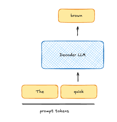
Speculative Decoding is a technique where you use a small draft model to propose a likely draft sequence, and then you use your big model to verify that sequence in parallel (in a single forward pass).
Traditional LLM decoding goes one token at a time.
But speculative decoding allows you to look at many tokens at once, and accept the ones that would have been generated by the big model.
Types of Work
When a model runs on a GPU, there are different types of work going on. The obvious one is running the matrix multiplies, dot products, or other tensor operations. But an important less obvious one is: loading data from global memory to local memory (and vice versa).
When the GPU is waiting on data to load for an operation, we call that a memory bound operation. If everything is loaded but we’re waiting on all the tensor operations to finish, we call that a compute bound operation.
When an LLM is decoding one token at a time, it is very memory bound. For every token we have to stream all the active parameters of the model. When an LLM is doing a batched decode of thousands of tokens in a single step, it’s compute bound.
When LLM decoding is memory bound, you’re wasting compute. The GPU could be doing more operations, but it’s not. For instance, if you were decoding 2 sequences instead of 1, it wouldn’t take any more time per token.
Speculative decoding is a way of using that extra compute to make decoding faster (at low batch sizes).
Trading Breadth for Depth
To make this concrete, let’s say the optimal number of tokens to run is 5 in a given forward pass. If we ran any fewer, we’d be memory bound, any more and we’d be compute bound.
We have two options.
First, we can run a batch size of 5 sequences, each decoding one at a time. We’ll say this is “breadth” (across sequences).
Alternatively, we can use speculative decoding to run 5 tokens in one sequence, achieving high “depth” for that sequence.
In both cases, the GPU is doing roughly the same amount of work. In the first case, all 5 sequences make a little bit of progress, in the second, our one sequence makes a lot of progress.
If you add more sequences and speculate to the same depth, you’ll just be slowing them all down as you’re compute bound.
But at small batch sizes (where batch size << optimal number of tokens), speculative decoding allows you to use “free” compute to complete all the sequences faster!
Why Does This Matter?
This might all sound a little pedantic. Speculative decoding does make things faster at small batch sizes, so who cares if it’s as much or more work?
This becomes important when you start to serve real-world loads or digging into speculative decoding research. If the optimal batch size is 5 but we’re running with speculative decoding on, we’re actually wasting compute when we could be using that time to move memory!
Especially if our acceptance rate isn’t 100%, every rejected token is extra wasted work.
This is why, at high throughput, vLLM gives you the configurability to totally turn off speculative decoding with the --speculative-disable-by-batch-size param.
And researchers looking at this picture started to wonder: why would we speculate to the same depth at every timestep? Why not speculate deep when we have extra compute (small batch size), and shallow, or even dynamically per sequence, when we have a larger batch size:

ATLAS: Evaluating Agents on Search-Intensive Tasks
Exa released ATLAS, a new benchmark designed to evaluate search-intensive agents on unmemorized, real-world research tasks.
Deep dive
- Dataset Scope: Features 547 deep research tasks requiring 2–10 multi-hop attributes per entity.
- Evaluation Metric: Uses three F1 metrics: Discovery (finding rows), Row (all cells correct), and Item (cell accuracy).
- Cost Efficiency: Grading an entire suite costs ~$0.24, significantly cheaper than LLM-judge benchmarks like WANDR.
- Reliability: Audit of the golden key shows less than 1% error rate, verified by manual human intervention.
- Search Bottleneck: The benchmark demonstrates that model intelligence is currently less of a bottleneck than search retrieval quality.
Decoder
- Row F1: A scoring metric that counts a result as correct only if all attributes in a row are perfectly matched.
- Multi-hop: A search pattern where an agent must follow links or perform subsequent searches to gather linked information across multiple domains.
Original article
Today we’re previewing ATLAS, a new benchmark designed to grade the accuracy and completeness of agent responses to challenging real-world workflows that heavily utilize web search. ATLAS pairs queries grounded in real search demand with verified golden answers, using an automated pipeline that lets us refresh both as the web and models evolve.
Some of our takeaways from our runs of ATLAS to date:
- Comprehensive search at a reasonable cost is far from solved. Max-effort search agents consistently outperformed their lower-compute counterparts, but no agent run costing less than $1 per task achieved a row F1 over 0.5.
- Even the most expensive search agents miss about 1/3 of the golden results, indicating substantial room for web search to improve performance in use cases where completeness is critical.
- When holding the model harness fixed, Exa defines the cost-performance Pareto frontier, with scores ranging 16% across different search backends.
What does a good benchmark look like?
When language models first started using web search, they would often get stuck managing long contexts or reasoning across multiple documents. Even the order of search results could throw them off. In short, agentic search was bottlenecked by intelligence. Now, frontier models handle these tasks much more reliably and at a fraction of the cost, so the bottleneck to completing deep and wide research tasks is whether your search backend can actually find relevant information in the world.
Recent bake-offs between agentic search configurations reflect the increasingly urgent need to rigorously evaluate web search efficacy. These evaluations seek to elucidate which combinations of harness, model, and search provider work best on challenging and economically valuable research tasks.
To support rigorous comparisons, we think an agentic search benchmark should:
- Require search. Answers must depend upon retrieving information from sources beyond what models already have memorized.
- Reward search quality and effort. High-quality search results and additional search volume should meaningfully improve scores.
- Represent real-world search tasks. Tasks must reflect what humans and agents actually search for.
These requirements may sound obvious, but today’s popular agentic-search benchmarks each fail one or more of them. Newer benchmarks stay fresh by grading with an LLM judge, which makes runs expensive to grade and highly sensitive to grader design.
These benchmarks tend to lose value over time as search providers optimize for them and the knowledge they require gets added to the latest frontier models. These issues are all downstream of the fundamental challenge that building new, high-quality search evals is slow and expensive. Therefore, agentic search benchmarks often go stale faster than they are replaced with fresh, up-to-date ones.
Designing ATLAS
We address these shortcomings with a new benchmark, ATLAS (Agentic Tasks for Large Aggregation + Search), consisting of 547 deep and wide research tasks. Tasks are generated from seed topics drawn from clustering of anonymized search demand. Each task asks a system to discover every entity (e.g. a person, place or company) that meets precise conditions, and then to enrich each entity with 2–10 multi-hop attributes.
Following a growing trend of synthetically generated benchmark data, we expend extensive inference-time compute within a structured pipeline to generate tasks and golden answers. Our pipeline includes a committee of frontier models and search providers which spend a median of 8 agent-hours and 1,200 searches per task to find answers, independently verify them against sources, and resolve disagreements or ambiguities until confident in their correctness. Because the pipeline is automated, we can regenerate the ATLAS dataset using topics based on recent search trends, keeping the benchmark aligned with what agents actually search for as the web updates.
Given the large amount of inference-time compute deployed at eval generation time, the challenge we pose for this benchmark is efficient search: solve each task in under a minute and for under $1, a budget at which no current system reaches even 0.5 row F1.
Results
Based on a suite of ablations and experiments, we believe that ATLAS rectifies the multitude of flaws present in current popular agentic search evals, providing a benchmark that truly measures search and distinguishes various systems by search quality and effort.
ATLAS strongly differentiates search providers.
ATLAS rewards search quality
ATLAS depends on search quality far more than existing benchmarks: when we severely degrade the quality of search by hiding the top 7 of every 10 search results, the same searcher loses roughly half of its ATLAS score. In contrast, on other benchmarks, the searcher retains 81–89% of its original score, indicating that these benchmarks do not actually measure search quality.
ATLAS is unmemorized
We measure memorization of evals by checking the percent of tasks whose full answer set is recalled by at least one of the major frontier models. Nearly 50% or more of other popular benchmarks are memorized.
In contrast, ATLAS’s older rows are less memorized, and it includes fresh information past current frontier model knowledge cutoffs, where frontier models almost never answer correctly without search. As a result, adding search to frontier models gives a much bigger lift in performance over a no-search baseline than current popular evals.
ATLAS requires wide and deep search
74% of ATLAS’s tasks ask for 10 or more entities, and each entity needs 2–10 attributes. Moreover, these wide and deep tables actually require multi-hop searches as opposed to retrieval from a single URL or domain. We estimate, based on our dataset construction logs, that discovery of entities requires a median of 4 different domains per task and full discovery + enrichment requires a median of 18 different domains per task.
Construction and validation
Two agents from different model families do the construction: Codex with GPT-6 Astra and Claude Code with Opus 5.5. To ensure the gold is not biased towards any one search index, every agent searches through a provider-neutral tool we built.
1. Topic seeding
Each task starts from a topic in Exa’s aggregate, anonymized search demand. Seeding from real demand spreads ATLAS across more than 300 topics and increases the likelihood that proposed tasks are unmemorized.
2. Entity discovery
The two construction agents search independently over several passes to construct a golden list of entities. A verifier agent then point-wise checks every row, including its cited pages, with additional searches on a separate index. Any unsettled rows go to targeted repair.
3. Row enrichment
After the discovery entity list is established, an agent proposes enrichment columns. The two construction agents fill every cell independently, saving each value with a page citation and a verbatim quote. Verification, repair and a final checker then settle any disagreements.
Grading
We grade returned tables against golden answers using three F1 metrics, computed per task and averaged over tasks. Each F1 is the harmonic mean of precision and recall.
- Discovery F1 counts just row discovery.
- Item F1 counts cells, including both discovery and enrichment.
- Row F1 counts rows, where a row is correct only when every cell in the row is. This is our headline metric.
The grader aligns returned rows to the key by entity name and a set of aliases, falling back to an LLM aligner on misses. Grading is both cheap and consistent.
Driving future innovation
We believe that ATLAS provides a much more faithful signal than existing benchmarks of which agentic search configurations actually work on hard, economically valuable research. As reflected in initial runs on ATLAS, efficient agentic search remains far from solved.
Exa will continue to push the frontier of efficient search toward solving wide and deep research at low latency and cost. We view ATLAS as a first step toward a new generation of continuously refreshed search evals, and we hope it helps measure progress on the workflows for which people actually rely on agentic web search.
Citation
@online{exa2026atlas, author = {Alexander Goldberg and Joshua Ahn and Scott Langille}, title = {{ATLAS: Evaluating Agents on Search-Intensive Tasks}}, date = {2026-10-08}, url = {https://exa.ai/blog/atlas-benchmark}}Quicksand (GitHub Repo)
Quicksand is an asynchronous Python API that simplifies managing QEMU-based Linux virtual machine sandboxes for AI agents without requiring root or Docker.
Decoder
- QEMU: A generic, open-source machine emulator and virtualizer.
- SLIRP: A user-mode networking implementation for QEMU that allows guest OSs to access the internet via the host's network stack without root access.
Original article
Quicksand
Quicksand is an async Python API to launch, control, and snapshot QEMU virtual machines with a particular focus on sandboxing AI agents. Quicksand provides pre-built Linux VMs for Ubuntu and Alpine distros and supports x86_64 and ARM64 across macOS, Linux, and Windows. Running sandboxes needs no root privileges or Docker; install the QEMU and image extras for a bundled runtime on supported platforms.
Installation
pip install 'quick-sandbox[qemu,alpine]'Or install the core package and add QEMU/images separately:
pip install quick-sandbox
quicksand install qemu alpine
Usage
Hello, World!
import asyncio
from quicksand import Sandbox

async def main():
    async with Sandbox(image="ubuntu") as sb:
        result = await sb.execute("echo 'Hello from the sandbox!'")
        print(result.stdout)

asyncio.run(main())
Run commands
result = await sb.execute("apt update && apt install -y python3")
print(result.stdout, result.exit_code)
Mount host directories
Share host directories into the VM at boot or on the fly.
# At boot
async with Sandbox(
    image="ubuntu",
    mounts=[Mount("./workspace", "/mnt/workspace")],
) as sb:
    ...

# Or dynamically on a running sandbox
handle = await sb.mount("/tmp/data", "/mnt/data")
await sb.execute("ls /mnt/data")
await sb.unmount(handle)
Configure networking
Sandboxes are network-isolated by default. Opt in to internet access and port forwarding with NetworkMode.FULL.
async with Sandbox(
    image="ubuntu",
    network_mode=NetworkMode.FULL,
    port_forwards=[PortForward(host=8080, guest=80)],
) as sb:
    ...
Multiple Linux users
Give multiple agents independent Linux user accounts in a single sandbox VM.
async with Sandbox(image="ubuntu") as sb:
    alice = await sb.create_user("alice")
    bob = await sb.create_user("bob")

    await alice.execute("cat > hello.txt", stdin="Hello from Alice!\n")
    await bob.execute("cat > hello.txt", stdin="Hello from Bob!\n")

    for user in (alice, bob):
        result = await user.execute("whoami && pwd && cat hello.txt")
        print(result.stdout)
        await sb.delete_user(user.name)
Save and load
Save the VM's disk state to a directory. Load it later, even on a different machine.
await sb.execute("pip install numpy pandas")
await sb.save("my-env")  # VM keeps running

# Load later
async with Sandbox(image="my-env") as sb:
    await sb.execute("python3 -c 'import numpy; print(numpy.__version__)'")
Checkpoint and revert
Capture the full VM state and roll back if something goes wrong.
await sb.checkpoint("before-experiment")
await sb.execute("apt install -y something-risky")
await sb.revert("before-experiment")  # the VM snaps back to the checkpoint
Control a desktop
Desktop images provide a full Xfce4 graphical environment with a browser. Install one with quicksand install ubuntu-desktop or quicksand install alpine-desktop.
async with Sandbox(image="ubuntu-desktop", enable_display=True) as sb:
    await sb.screenshot("screen.png")
    await sb.type_text("hello world")
    await sb.press_key(Key.RET)
    await sb.mouse_move(500, 300)
    await sb.mouse_click("left")
Configuration
Here are all of the Sandbox configuration options:
Sandbox(
    # Image or save name to boot
    image="ubuntu",
    # Guest RAM (default: "512M")
    memory="2G",
    # Virtual CPU cores (default: 1)
    cpus=4,
    # Host directories shared into the VM at boot
    mounts=[Mount("/host", "/guest")],
    # NONE, MOUNTS_ONLY (default), or FULL internet access
    network_mode=NetworkMode.FULL,
    # Forward host TCP ports into the guest
    port_forwards=[PortForward(host=8080, guest=80)],
    # Expand the guest filesystem on boot
    disk_size="10G",
    # Attach virtual GPU, keyboard, and mouse for screenshot/type_text/mouse control
    enable_display=True,
    # Auto-save VM state on stop
    save="my-save-name",
)
Available images
| Image | Type | Wheel size | Install command | What is it |
|---|---|---|---|---|
ubuntu |
Base | ~309-357 MB | quicksand install ubuntu |
Ubuntu 24.04 headless |
alpine |
Base | ~82-85 MB | quicksand install alpine |
Alpine 3.23 headless (faster boot) |
ubuntu-desktop |
Overlay (ubuntu) |
~273-281 MB | quicksand install ubuntu-desktop |
Ubuntu 24.04 + Xfce4 + Firefox |
alpine-desktop |
Overlay (alpine) |
~346-363 MB | quicksand install alpine-desktop |
Alpine 3.23 + Xfce4 + Chromium |
quicksand-agent |
Overlay (ubuntu) |
~306-335 MB | quicksand install quicksand-agent |
Ubuntu + Python 3.12, uv, build-essential, requests, pyyaml, ddgs, markitdown |
quicksand-cua |
Overlay (quicksand-agent) |
~489-500 MB | quicksand install quicksand-cua |
Agent Sandbox + Xvfb, x11vnc, noVNC, Playwright, Chromium |
Sizes are approximate full image-wheel downloads for the September 14, 2026 releases and vary by architecture. Overlay sizes exclude their base images.
Building from source
git clone https://github.com/microsoft/quicksand.git
cd quicksand
uv sync
uv run uvr build --all-packages
Documentation
| Topic | Guide | Under the Hood |
|---|---|---|
| Installation | Installing packages | QEMU binaries, kernels, qcow2 disks |
| Sandbox Lifecycle | Creating and configuring sandboxes | -m, -smp, -accel, machine types |
| Running Commands | execute(), streaming, exit codes |
Kernel boot, agent tokens, hostfwd |
| File Exchange | Mounts, hot-mounts, getting data in/out | CIFS via guestfwd, 9p via -fsdev |
| Save and Rollback | Checkpoints, reverts, persistent saves | qcow2 overlays, savevm, blockdev-snapshot-sync |
| Desktop Control | Screenshots, keyboard, mouse | VNC, GPU, USB tablet, QMP input injection |
| Network and Isolation | Network modes, port forwarding | SLIRP NAT, restrict=on, guestfwd |
| Performance | What makes it fast | io_uring, IOThreads, TCG vs KVM |
Contributing
| Guide | When to use |
|---|---|
| Creating Images | Build a new base or overlay image package |
| Extending the Sandbox | Add a method, OS, architecture, or QEMU flag |
| Testing | Run or write tests |
| Releasing | Cut a release |
NVIDIA's Long-Video and World-Action Research (GitHub Repo)
NVIDIA released LongLive 2.0, a parallel infrastructure for real-time interactive long-video generation using NVFP4 quantization to achieve up to 45.7 FPS.
Decoder
- NVFP4: A 4-bit floating point format used by NVIDIA to accelerate deep learning inference and reduce memory bandwidth requirements.
- KV Cache: A technique in transformer models that stores previously computed key and value vectors to avoid redundant calculations during token generation.
- Attention Sink: A mechanism that designates certain tokens to capture high-intensity attention scores, preventing instability in long-sequence models.
Original article
🎬 LongLive 2.0: An NVFP4 Parallel Infrastructure for Long Video Generation
Paper Code Video Models Models Demo Docs
💡 TLDR: Infra with NVFP4 and parallelism for both training and inference
News
- 🔥 [2026.05.13] We release LongLive 2.0, infra with NVFP4, parallelism and multi-shot for AR training, DMD distillation, and inference (⚡45.7 FPS). The original LongLive 1.0 is now in the v1.0 branch.
- 🔥 [2026.04.12] LongLive supports kv cache compression with TriAttention, with 50% KV reduction and no quality drop. Check it here
- 🎉 [2026.1.27] LongLive is accepted by ICLR-2026.
- 🔥 [2026.1.11] LongLive supports adapting LongLive's original RoPE into KV-cache relative RoPE and generates infinite long videos!
- 🔥 [2025.11.3] We implement LongLive on linear attention model SANA-Video! Now SANA-Video can generate 60s interactive videos in real-time.
- 🔥 [2025.9.29] We release Paper, this GitHub repo LongLive with all training and inference code, the model weight LongLive-1.3B, and demo page Website.
Introduction
LongLive 1.0: Real-time Interactive Long Video Generation. You can find it here in our V1.0 branch.
LongLive 2.0: an NVFP4 Parallel Infrastructure for Long Video Generation
- For training, it supports
- Balanced sequence parallel for AR training (teacher-forcing).
- AR training on multi-shot (or single-shot) videos.
- NVFP4 (or BF16) for both AR training and few-step distillation.
- For inference, it supports
- NVFP4 inference (W4A4) and NVFP4 KV Cache.
- Multi-shot attention sink.
- Sequence parallel inference.
- Async decoding.
LongLive 1.0: Real-time Interactive Long Video Generation. It accepts sequential user prompts and generates corresponding videos in real time, enabling user-guided long video generation. The key insights are attention sink, KV-recache, and streaming long tuning.
Getting Started
Quick Start
BF16
import torch
from omegaconf import OmegaConf

from pipeline import CausalDiffusionInferencePipeline
from utils.config import normalize_config
from utils.inference_utils import (
    load_generator_checkpoint,
    place_vae_for_streaming,
    prepare_single_prompt_inputs,
    save_video,
)

prompt = "A compact silver robot walks through a clean robotics lab."
merged_checkpoint_path = "LongLive-2.0-5B/model_bf16.pt"

config = normalize_config(OmegaConf.load("configs/inference.yaml"))
device = torch.device("cuda")

torch.set_grad_enabled(False)
pipe = CausalDiffusionInferencePipeline(config, device=device)
load_generator_checkpoint(pipe.generator, merged_checkpoint_path)
pipe = pipe.to(device=device, dtype=torch.bfloat16)
place_vae_for_streaming(pipe, config)  # honor streaming_vae + vae_device when set
pipe.generator.model.eval().requires_grad_(False)

noise, prompts = prepare_single_prompt_inputs(config, prompt, device)
video = pipe.inference(noise=noise, text_prompts=prompts)
save_video(video[0], "videos/quickstart/sample.mp4", fps=24)
place_vae_for_streaming is a no-op unless inference.streaming_vae is true and inference.vae_device is set, so toggling streaming-pipeline decode in your yaml is enough — the script does not need to change.
NVFP4
Point checkpoints.generator_ckpt in configs/nvfp4/inference_nvfp4.yaml at the downloaded checkpoint and set model_quant_use_transformer_engine according to the backend you are using:
- TransformerEngine checkpoint (
model_te.pt):model_quant_use_transformer_engine: true - FourOverSix checkpoint (
model_4o6.pt):model_quant_use_transformer_engine: false
setup_nvfp4_pipeline handles checkpoint loading, NVFP4 module wrapping, weight materialization, dtype/device placement, and the streaming-pipeline VAE relocation for both backends — the bf16 pipe.to(...) shortcut is unsafe here because it would cast the quantized buffers.
import torch
from omegaconf import OmegaConf

from pipeline import CausalDiffusionInferencePipeline
from utils.config import normalize_config
from utils.inference_utils import prepare_single_prompt_inputs, save_video, setup_nvfp4_pipeline

prompt = "A compact silver robot walks through a clean robotics lab."

config = normalize_config(OmegaConf.load("configs/nvfp4/inference_nvfp4.yaml"))
device = torch.device("cuda")

torch.set_grad_enabled(False)
pipe = CausalDiffusionInferencePipeline(config, device=device)
setup_nvfp4_pipeline(pipe, config, device)
pipe.generator.model.eval().requires_grad_(False)

noise, prompts = prepare_single_prompt_inputs(config, prompt, device)
video = pipe.inference(noise=noise, text_prompts=prompts)
save_video(video[0], "videos/quickstart/sample_nvfp4.mp4", fps=24)
Models
| Model | FPS ↑ | Params | VBench ↑ | Multi-shot |
|---|---|---|---|---|
| LongLive-1.3B | 20.7 | 1.3B | 84.87 | |
| LongLive-2.0-5B | 24.8 | 5B | 85.06 | ✅ |
| LongLive-2.0-5B-NVFP4-4Step | 29.7 | 5B | 84.51 | ✅ |
| LongLive-2.0-5B-NVFP4-2Step | 45.7 | 5B | 83.14 | ✅ |
License
This repository is released under the Apache 2.0 license. See LICENSE for details.
Citation
Please consider citing our work if you find them useful:
@article{longlive_2.0,
  title={LongLive2.0: An NVFP4 Parallel Infrastructure for Long Video Generation},
  author={Chen, Yukang and Wang, Luozhou and Huang, Wei and Yang, Shuai and Zhang, Bohan and Xiao, Yicheng and Chu, Ruihang and Mao, Weian and Hu, Qixin and Liu, Shaoteng and Zhao, Yuyang and Mao, Huizi and Chen, Ying-Cong and Xie, Enze and Qi, Xiaojuan and Han, Song},
  journal={arXiv preprint arXiv},
  year={2026}
}
@inproceedings{longlive,
    title={Longlive: Real-time interactive long video generation},
    author={Yang, Shuai and Huang, Wei and Chu, Ruihang and Xiao, Yicheng and Zhao, Yuyang and Wang, Xianbang and Li, Muyang and Xie, Enze and Chen, Yingcong and Lu, Yao and others},
    booktitle={ICLR},
    year={2026},
}
Acknowledgement
- Self-Forcing: the AR training codebase and formulation we build upon.
- Wan2.2: the base video diffusion model components used in this release.

Anthropic Cyber Defense Initiative
Anthropic is launching its 'Cyber Mission' to deploy frontier models, engineering talent, and automated vulnerability scanning for critical infrastructure and open-source projects.
Decoder
- Operational Technology (OT): Hardware and software systems that detect or cause a change through the direct monitoring and control of physical devices like power grids or factory equipment.
Original article
Introducing the Anthropic Cyber Mission
Today we’re launching the Anthropic Cyber Mission, a long-term commitment to securing the systems everyone depends on. The Cyber Mission is a new effort to support defenders with tools, research, and resources to secure their software and systems. We’re starting with two areas:
- Critical infrastructure: Starting with securing the operational technology behind power grids, water systems, and transportation networks, and protecting government systems. Today, we’re introducing the Critical Infrastructure Defense Program (CIDP), which brings frontier models, on-site engineers, and threat research to the defenders that protect operational technology.
- Open-source software: Finding vulnerabilities and proposing patches in the free, shared code that most software depends on, and hardening the underlying code. Today, we’re launching OSS Scanner, which offers open-source projects regular security scans from our strongest models, for free.
Frontier models can be misused to exploit vulnerabilities and conduct cyber operations. Despite best efforts, many areas of technology remain dangerously exposed. State-sponsored adversaries have spent years gaining footholds in these systems, across many sectors, so that they can disrupt them. Defenders of critical infrastructure and the OSS community have decades of security experience but have faced severe resource shortages that are exacerbated by this moment. We are recognizing their expertise in these domains and offering our support. We will also expand the Cyber Mission to release tools, research, and resources in new areas to help secure the world.
As part of Project Glasswing, partners uncovered many vulnerabilities, but we haven’t yet achieved a sufficient reduction in cyber risk. It’s easier than ever to find vulnerabilities, but verifying, prioritizing, and fixing these findings remains challenging. Based on lessons from Project Glasswing, we’re starting these new efforts to support defenders. Earlier this week, we merged Project Glasswing into our expanded Cyber Verification Program, which gives many more defenders access to our most capable models. And through the Anthropic Cyber Mission, we’ll deploy Anthropic engineering talent and provide tools and funding for those who secure critical infrastructure and open-source software.
Defending critical infrastructure
Power grids, water utilities, factories, and transportation networks run on controllers, control software, and industrial networks built to last for decades. These systems are known as “operational technology,” and they often cannot be taken offline to patch, so known vulnerabilities can stay unresolved for years. Securing them is specialized work: the equipment is proprietary, changes are risky, and a mistake can take down a plant. Operators of every size rely on a small set of trusted providers to support that work, telling them what’s exposed and which fixes to make on a running system.
Today, we’re introducing the Critical Infrastructure Defense Program, which brings frontier Claude models, on-site engineers, and our threat research to those trusted providers. Its founding partners are Accenture, Booz Allen, CrowdStrike, Deloitte, Dragos, Hitachi, Insane Cyber, Nozomi Networks, Palo Alto Networks, PwC, and Rockwell Automation.
These organizations represent the providers that operators rely on to secure these systems: the consulting and advanced technology companies that run security programs, the security companies that guard the business and industrial networks, and the manufacturers that build and patch the equipment itself.
This work is underway. Several partners are currently working with Claude to fix vulnerabilities and help customers do the same. Critical infrastructure is hard to defend in many ways that AI cannot fix, but we believe that frontier models can help find and repair weaknesses before those weaknesses are used to cut off power or make water unsafe. Our first step is to work with a small cohort of providers to learn which strategies are most effective and practical.
If your company builds security products or services for critical infrastructure, you can register your interest here.
As AI continues to advance, it presents an important opportunity to strengthen cybersecurity across critical infrastructure, provided it is applied responsibly, validated rigorously, and deployed with safety and reliability at the forefront. We are pleased to contribute our operational technology and industrial cybersecurity expertise to help develop practical approaches for applying AI in ways that strengthen the resilience of the infrastructure society depends on every day.
Through our work with critical infrastructure organizations, PwC’s cyber OT practice has seen firsthand the gravity of consequences cyber breaches can have in these environments. I firmly believe that a coordinated, industry-wide effort is necessary to identify vulnerabilities, mitigate risks, and strengthen the resilience of our critical systems.
Threat actors are using AI to find and exploit exposures at machine speed. By combining Unit 42 threat intelligence and operational expertise with Anthropic’s frontier models, we’re helping operators defend against adversaries looking to attack and disrupt essential services. Together, we are giving defenders the speed and precision needed to close attack paths before exposure becomes impact.
Frontier AI is evolving faster than any single organization can track alone. That’s why the Critical Infrastructure Defense Program matters. It brings together the people who understand these environments with the frontier capabilities now available to defend them. We’re proud to contribute our experience and to learn alongside the other partners working to protect the systems the world depends on.
The sites that need protection most, like remote substations, offshore platforms, and air-gapped plants, are exactly where traditional tools can’t reach and specialists can’t be. What no one had solved was the hours: more data than any team can work through, at more sites than any team can staff. Claude closes that gap, so our analysts and our customers’ operators spend their time on the judgment calls that keep critical systems running safely.
Critical infrastructure and the people who depend on it benefit when the vendor community shares what they learn about the opportunities and challenges that AI presents to operational environments, rather than keeping that knowledge in silos. Joining Anthropic's Critical Infrastructure Defense Program is one of the ways we help align frontier AI to a collective defense strategy built around the realities of the operational technology (OT) that keeps the lights on, water safe, and transportation running.
Critical infrastructure is where cyber risk becomes real-world risk. As adversaries use AI to move faster and operate at greater scale, critical infrastructure facing machine-speed threats requires machine-speed defense. By bringing CrowdStrike’s deep security context and expertise together with Anthropic’s frontier AI expertise, we can put a greater advantage in the hands of critical infrastructure defenders.
Amid the rapid evolution of AI and the increasing sophistication and speed of cyber threats, ensuring cybersecurity in OT environments that support social infrastructure has become one of the highest priorities facing society today. Through participation in this program, we look forward to collaborating with Anthropic and fellow partners to further enhance cyber resilience for critical infrastructure.
As AI accelerates, critical infrastructure operators need solutions that address security vulnerabilities at machine speed. Together with Anthropic, Deloitte is helping provide these enterprises with the enablement needed to close security gaps and strengthen resilience, moving at pace with the realities of frontier AI.
Operational technology is the next frontier for autonomous AI-enabled attacks. The question is no longer whether AI can affect an industrial process, but how much control it can gain, and how quickly. The Critical Infrastructure Defense Program is convening the best of private-sector innovation and investment to strengthen OT and ICS resilience across federal and commercial missions.
Organizations that keep our power on, medicine safe, food supply secure, and communications running face some of the most consequential cyber risks in the world. Accenture is committed to bringing our deep OT security expertise to the organizations that protect the critical infrastructure communities depend on every day. This partnership will help put AI-powered defense in the hands of those who need it most.
In June, we launched a cyber defense program for state, local, tribal, and territorial governments. Since then, we’ve offered frontier Claude models and technical support to more than half of all US states and some of the country’s largest public critical infrastructure operators, speeding up code scanning and patching, incident response, red teaming, and other security workflows.
We are listening to and learning from the people who know this landscape best. Our approach is to work with the companies, coalitions, governments, and nonprofits that know this landscape and that operators trust, and provide support where it’s most needed.
Securing open-source software
Almost all software relies on open-source code, much of it maintained by small teams of volunteers. Under Project Glasswing, we scanned hundreds of widely used open-source projects, had humans triage and review many of the potential vulnerabilities uncovered, and privately reported what we found to their maintainers through our coordinated vulnerability disclosure process.
Some maintainers with the capacity to triage at scale asked us for everything our models had found in their project, reviewed or not. In response, we’re launching OSS Scanner, an opt-in service inspired by Google’s OSS-Fuzz. Enrolled projects receive periodic scans from our most capable models, free of charge. Each report includes a proof of concept of how the bug could be exploited, an explanation, and a suggested fix where one is available. The reports are model-generated and sent without human review. That means maintainers receive them faster, but it also means that some will contain inaccuracies, such as a wrong severity rating. We expect a true-positive rate above 90%, and will work to improve the true positive rate and fix quality over time. The team’s post explains how it works and how to enroll.
The service is meant for projects with the capacity to keep up with surfaced findings. For others, we will continue to share human-verified disclosures under our CVD policy.
OSS Scanner is a first step. From here, our open-source work aims to:
- Get findings to maintainers faster. Bring OSS Scanner to more projects while keeping human-verified disclosure for those that need it.
- Accelerate fixes. Automate triage and patching, which are still mostly manual, for projects that want it.
- Explore new secure architectures and coding practices. Research and share methods for hardening or rewriting code with projects that want to go further than patching.
We’ll do this based on guidance from open-source maintainers and foundations, and share what works so other projects can replicate it. We funded the organizations behind widely used open-source code, including the Python Software Foundation, Alpha-Omega and OpenSSF through the Linux Foundation, and the Apache Software Foundation, as well as supporting Akrites and Gold Eagle, which collect and coordinate vulnerability reports from many sources to avoid overwhelming maintainers. The Defender Advantage Fund (0xDAF), which we launched in August, supports pilot programs in these areas and keeps OSS Scanner free.
Maintainers can also apply to Claude for Open Source for free Claude Max subscriptions, and to the Cyber Verification Program for expanded access to Claude’s cyber capabilities for defensive work.
Why we're doing this
Highly cyber-capable AI models are widely available to attackers now. But defensive tools—including our own—have not yet reached enough of the defenders who need them. OSS Scanner, our Cyber Verification Program, defensive products our partners build on our platform, and Claude Security are some of our efforts here, and we’ll be adding others as soon as possible.
Our forecast is that in two years, AI will favor defense: it will be easier to catch bugs before they ship, write fundamentally secure software from scratch, and actively defend systems with models. But in the near term, that may not be true. The cost of exploiting vulnerabilities has dropped, while verifying, disclosing, and fixing them is slow and still depends on people. In Glasswing, we often saw months pass between a vulnerability being found and being fixed. With operational technology, a fix may have to wait until it can be applied safely to running machinery—in some rare cases, this might take decades.
Success means critical infrastructure such as water, power, transport, and communications keep running in the face of attacks by capable adversaries, with fewer exploitable paths in and faster recovery when something gets through. This will take years and we expect the Anthropic Cyber Mission to change as we, together with the public and private sector, learn what works.
The path ahead
Over the coming months, we’ll bring the Critical Infrastructure Defense Program to more partners and more sectors, and we’ll share what we learn along the way, including what didn’t work. We also expect other AI developers, security companies, and governments to run efforts of their own, and we’d like to collaborate with them wherever that helps defenders.
We will also expand our work to help secure open source and the broader supply chain. This includes researching new ways of writing software and new ways of defending systems. We intend to share frontier research, tools, and resources to help others secure their software and supply chain.
If you’d like to work with us:
- Companies that build security products or services for critical infrastructure, including security vendors, system integrators, and equipment manufacturers, can register their interest in the Critical Infrastructure Defense Program as we expand it.
- Core maintainers of critical open-source projects can enroll in OSS Scanner.
- Security teams of any size, including operators of critical infrastructure and open-source maintainers, can apply to our expanded Cyber Verification Program for access to our models.

The Return of Wake-Sleep
Harvey’s research demonstrates that a wake-sleep agent training loop can boost all-pass performance on legal tasks from 2.9% to 15.7%.
Deep dive
- Methodology: Used 196 tasks from the Legal Agent Benchmark (LAB).
- Performance: Increased pass rates across both familiar and new, unseen legal matters.
- Feedback Loop: Used dual LLM judges to grade performance without the agent seeing the grades, ensuring unbiased evaluation.
- Knowledge Synthesis: Sleep phase distilled raw trajectories into reusable checklists and best practices.
- Optimization: Memory retrieval reduced token costs by 50% while maintaining performance by selecting only relevant lessons per task.
Decoder
- Wake-sleep: A machine learning algorithm where the agent learns online (wake) and then uses its experience to generate and refine knowledge offline (sleep).
- Held-out tasks: Data points withheld from the training phase to test the agent's ability to generalize to new information.
Original article
The Return of Wake-Sleep
Wake-sleep is a classic learning algorithm that trains an AI system by alternating between two phases. In the wake phase, the system acts online and observes real data, such as images, audio, or text. In the sleep phase, it "dreams up" examples offline that might improve online behavior. While originally introduced to train neural networks, later systems used the same concept to build up reusable knowledge (e.g. DreamCoder, LILO and DreamProver).
As production, knowledge-intensive agent use cases proliferate, hybrid online-offline protocols like wake-sleep are increasingly becoming a part of the agent stack. Long-horizon agents now work on individual tasks for hours. As these agents work, they leave a record of actions and deliverables, and with the right verifiers we can tell which actions led to good deliverables and which fell short. That record can be reviewed offline, by LLMs or other agents, and transformed into memories or structured context that the agent can leverage on its next task.
Agent research has started moving in this direction, exploring a range of approaches for persisting notes, workflows, or playbooks across repeated agent interactions (see Reflexion, Agent Workflow Memory, Dynamic Cheatsheet, ACE, etc). Anthropic, with Dreaming in Claude Managed Agents, is a current leader in building frameworks for general-purpose agent context and "sleep-time" context management. Cognition also recently introduced dreaming in its Agent Memory Repo release.
Motivated by these directions, we explored how wake-sleep might apply to long-horizon legal agents. We evaluated our own variant of wake-sleep on tasks from Harvey’s Legal Agent Benchmark (LAB) and found that:
- Wake-sleep meaningfully improves agent performance on complex tasks.
- The memory and context written offline by the sleep phase generalizes to new matters and kinds of task the agent did not see in training.
- Allowing the agent retrieve only the memories relevant to each task, rather than reading all of them, halves the cost per task at about the same average quality.
Wake-sleep for legal agents
So what might a wake-sleep implementation look like for long-horizon agents? In our version of wake-sleep, each learning cycle proceeds through the following stages:
1. Agent rollout. In the wake phase, an agent works through a set of LAB tasks. Each task gives the agent instructions and a folder of documents from a synthetic client matter, and asks for a deliverable such as an issues list, a memo or a marked-up draft. The agent reads and searches across the documents, runs analyses, and writes and edits the final deliverables.
2. Grading. Dual LLM judges grade the deliverables against expert rubrics as in the standard LAB configuration. The agent does not see the grades.
3. Generate candidate lessons. In the sleep phase, a review model reads each graded training run, with the agent’s trajectory, its deliverables, and the verdict on every rubric criterion, and writes candidate lessons about what went wrong. A lesson is either a checklist item, which states something a deliverable must contain, or a practice note, which states how to do part of the work.
4. Merge. The review model then merges the candidate lessons into the agent's memory. It combines lessons that overlap, revises existing lessons and drops some. From the second cycle on, it also judges which existing lessons helped.
5. Commit. The biggest risk in lesson generation is overfitting—e.g. writing down facts specific to one training matter, such as a party’s name or a purchase price, instead of learnings that carry to other matters. To prevent this, we implemented a commit gate that uses Jev to reject lessons that contain client-specific detail, are too narrow, or rest on a single training task. Rejected lessons go to a review queue and are not added to the memory.
6. Store. The memory stores the lessons as text, grouped by kind of work (analysis, drafting and review), with a fourth group for general learnings.
When initialized, the agent's memory contains no lessons or structured context. In each successive wake-sleep cycle, the agent's memory store is updated with the lessons and structured context it learned in the prior cycle.
Experiment and results
We ran a 10-cycle wake-sleep process across 196 tasks from LAB’s Corporate M&A and Capital Markets practice areas (110 for training, 86 for validation), using the steps described in the previous section. We then compared the rubric pass rates between the wake-sleep agent and a vanilla agent with no memory or internalized context across each of the tasks. For these initial experiments, GPT-6 Luna was used as the agent model.
To test generalization, we grouped hold-out tasks into two cohorts based on their distance to the training task distribution:
- Familiar matters: Tasks similar to those found in the training distribution, with similar document types and source instructions to the training tasks.
- New matters: Fundamentally different tasks than the agent encountered in the wake-sleep training cycles.
Results from these runs are shown in Figure 3. Overall, we found wake-sleep to improve performance significantly across all tasks, reaching 15.7% all-pass, up from 2.9% for a vanilla agent. These all-pass gains are attributable to a large increase in rubric-level pass rates across both of our experimental conditions, with the wake-sleep agent completing over 10% more rubric criteria per task on familiar matters, and nearly 5% more rubric criteria per task on new matters relative to the baseline agent.
Unsurprisingly, the biggest per-step gains come from the initial wake-sleep cycles, where the agent picks up its first lessons and best practices for legal knowledge work.
Qualitative Findings
To better understand the impact of wake-sleep, and the evolution of learned memory and context, we examined at agent behavior (online) and memory (offline) across each of the first 10 wake-sleep cycles.
In the first sleep cycle, the sleep process adds 122 lessons to agent memory. The majority of these initial lessons are checklist items that indicate what a high-quality deliverable must contain content-wise. Over the remainder of the sleep cycles, these lessons are refined into both behavioral best practices -- e.g., "When a term changes, explain how each alternative works" -- and tactical instructions -- e.g., "Recompute every figure yourself to verify it". Unhelpful or overly-specific lessons are pruned.
A qualitative example of this progression is shown in Figure 5, which follows one lesson about deadlines and time-related calculations that the agent learned and refined at sleep-time. In the first sleep cycle, the review model writes a rule to state contractual time terms as durations rather than start and end dates, with instructions on how to compute such durations:
State every contractual time term expressly as a duration, such as survival, lease term or notice period, not only as start and end dates. For every future deadline, compute the days remaining from the memo date, show the arithmetic, and put it in the bottom line or in the executive summary.
Over the next nine sleep cycles, the review model added a rule for each new case it met, such as a deadline that falls on a weekend or two documents that set different windows for the same delivery.
These lessons also change online agent behavior by influencing how the agent works, as shown in Figure 6. Using these lessons and best practices, the agent made ~2.5x more tool calls per task to run code, check its work, and draft and edit deliverables in accordance with its developing memory. The agent made about as many calls to read and search documents as before, indicating that these initial gains primarily target post-research work like analysis and writing. An interesting direction of future study is to identify lessons and best practices that improve agent behavior with respect to search and retrieval.
Importantly, this extra analysis and work-checking makes runs slower and more expensive. The wake-sleep agent is trading cost and latency for more thorough, higher-quality work, which raises the question of whether it can maintain that quality while working more efficiently.
Making wake-sleep more efficient
To improve the efficiency of wake-time agent behavior, we evaluated lesson retrieval. To implement this, we again use Jev, this time asking it if each lesson is relevant and helpful the task at hand. Only the lessons Jev judges most likely to help are injected into the agent's context.
We found that retrieving a fixed set of relevant lessons from the sleep bank halved the agent's cost per task while maintaining its rubric criteria pass rate. This suggests that wake-sleep, similar to other agent paradigms, benefits from online context management optimizations.
What we learned about wake-sleep for agents
Production agent deployments will increasingly combine online work with offline processing. Agents will act on tasks in real time, while background processes index documents, summarize past sessions and curate what the agent remembers. Algorithms like wake-sleep, which separate doing the work online from learning from it offline, are a natural next step for agent architectures.
In this work, we explored wake-sleep in a long-horizon legal agent setting, using primarily non-parametric forms of agent optimization (textual representations of context and best practices), but these techniques can be extended to parametric learning and post-training, as in the original wake-sleep formalization.
For verifiable knowledge-intensive work, this loop offers a way for agents to get better over time.
SpaceX Makes Big Play to Become a Wireless Carrier
SpaceX is spending $8 billion to acquire cellular spectrum, signaling a aggressive push to provide terrestrial mobile coverage via Starlink.
Decoder
- Spectrum: The range of radio frequencies used for wireless communication, which must be licensed from government entities to avoid signal interference.
Original article
SpaceX will pay investment firm Grain Management about $8 billion in cash for US cellular spectrum licenses. The licenses will be for the 800-megahertz band, which is tailored for wireless service from cellphone towers rather than satellites. SpaceX says the new spectrum will help cover places satellite links can't reach. SpaceX still needs some terrestrial infrastructure to use the spectrum for mobile coverage.
First look at Claude Code mods (spoiler: yes, use one now!)
Claude Code Mods allow developers to inject custom UI, tool rules, and interface behaviors directly into the agentic terminal environment.
Deep dive
- Interface Customization: Mods can redraw the Claude Code interface, resize panes, and share data across hooks.
- Use Cases: Hyperlinking ticket numbers, building deployment watchers, and implementing lock-and-queue systems for parallel testing.
- Agent Efficiency: Reduces the need for agents to handle trivial tasks like querying production databases by providing deterministic, safer tool wrappers.
Decoder
- Hook: A point in the agent lifecycle where custom logic can be triggered.
- MCP (Model Context Protocol): An open standard that allows AI agents to interact with data sources and tools across different platforms.
Original article
I have to say I was sceptical at first. "Mods" – we already had hooks, right, so what can be so special? I'm not going to retell what mods can do. Nor do I recommend reading through the manual. Instead, ask Claude this:
Claude Code has mods now. Given the workflows we usually use and the type of work we do here, what are some mods we could build that would be super useful?
And let it build some. The key is, they can do everything to your Claude Code and you don't need to know how they work.
These mods and OpenAI's Intelligent UI (released just now) are super interesting steps towards the Disposable Software direction some futurists are talking about. I'm sure Codex, Grok, Gemini and everyone and their mother will have mods very soon.
My first mods
This is how my terminal looks like now, when running a long-running workflow. You will notice the extra right-side pane, that does not look native to Claude Code. And my god, I can resize it with my mouse..
This mod works in two settings – one for each of the main workflows I described in detail in my previous post – for task preparation and for building.
This is an actual workflow that did task preparation (here only the pane is shown). This specific workflow took two hours to complete and this visualization makes the entire thing understandable with just a glance. Here's an animated sped-up gif of it.
Here's one real recording of the build workflow that writes code and deploys work. This workflow often has tens of discrete steps (like code reviews and fixes, checking something in dev or prod, data heals, merges, deploys etc). This creates a nice overview of it all.
The second thing I could fix now, was my long time feature request, to always have a hyperlink where Claude refers a Github issue. Of course Claude knows what #2443 (and three other ticket references it casually mentions) means, because it has the context, but I don't.
So now I have a mod for this.
Make it so that whenever I see a ticket number in the terminal, it is a hyperlink
Amazing!
Next mods for me
These are all suggestions by Claude, which I love a lot. I'll get to them soon, but I'm listing them here to share some inspiration.
- Jira-like task board in terminal, so I can skip going to Github issues
- Deploy watcher and status light
- Move a lot of prose and rules from
agents.mdinto deterministic checks - Safer tool for querying production data, no hand-assembling the SQL proxy
- A queue and lock for running parallel e2e tests. I really love this! Today, my parallel agent count is limited by how many agents can run the memory-intensive browser-based tests simultaneously. They rarely actually end up doing it at the same time, but limit needs to be there still. This mod would act as a queue with locks that would only start limiting agent counts when they actually want to run the tests at the same time.
Someone made a Jev-based model switcher. Somebody made a mod where you can play Doom in a terminal pane while you wait for the model.
Bootstrap 6 Alpha
Bootstrap 6 Alpha drops legacy browser support for modern CSS standards, moves to an ESM-only architecture, and adds LLM-friendly documentation.
Deep dive
- Modern CSS: Uses
light-dark(),:has(), container queries, and native `` elements, eliminating the need for polyfills or prefixes. - Build Tooling: Replaced Rollup/Babel with Rolldown, significantly streamlining the build pipeline.
- Architecture: ESM-only JavaScript means `
Decoder
- ESM (ECMAScript Modules): The official standardized modular system for JavaScript, allowing clean dependency management using import/export syntax.
- Token Maps: A CSS-focused approach to theme management using variables that can be modified without recompiling the entire framework.
Original article
On this page
Today we’re releasing the first alpha version of Bootstrap 6, a major overhaul to the project that modernizes and expands one of the most prolific open source design systems of all time. It’s been incredibly fun and rewarding to work on this over the past year, and I’m excited to share it with you.
Bootstrap 6 has been modernized from the ground up with the Sass module system, support for more native browser APIs and elements, ESM-only JavaScript plugins, and a slew of new CSS standards. We’ve broken this post into separate entries that we’ll publish one-by-one, starting with an overview of v6 and a spotlight on our new Sass & CSS implementation.
Hold up…
You’re probably asking yourself, “Wtf, new Bootstrap? What is this, 2015?” And I don’t blame you. It’s been all quiet on the Bootstrap front for a long time while I’ve focused on Pierre, especially with our work on Diffs, Trees, and Code Storage.
Throughout all of that, I’ve had several nagging ideas for Bootstrap despite humans not writing any more code thanks to AI. And yes, there are tons of design libraries from amazing developers now. Still, the reason we made Bootstrap in the first place has never been more relevant.
To help people build more software, faster and easier.
There’s never been more people building software than today, and I imagine that will continue to be true every day, for the rest of our lives. It’s already been installed over 1.75 billion times since its release in 2011. So, Bootstrap 6 is here to continue being an open source design system for anyone—human or AI, novice or pro.
We hope you love it, and thanks to everyone who’s supported the project over the years.
Community appreciation
Before we get to the good parts, I want to thank my co-maintainer, Julien, for all the amazing work he’s put into Bootstrap over the last couple of years. Without him, I’d be underwater on reviews, dependencies, migrations, and more. He’s an absolute legend and Bootstrap owes him a tremendous amount of gratitude and appreciation.
Huge thanks to everyone who contributed to the v6 development branch as well:
@julien-deramond @coliff @pricop @ThomasLandauer @Rishikesh183 @pardeyke @meenalsingh0 @ifer47 @Hashim1999164 @fauzan171 @claudiob @aljojoby9 @VividLemon @cccabinet @Rawal27 @jonnysp @kwy404 @andreas-venturini
And most importantly, thanks to everyone who has backed Bootstrap on Open Collective and every contributor who filed an issue, sent a patch, or argued with me in a pull request.
Get started
Bootstrap 6 Alpha 1 is on npm and jsDelivr right now.
npm i bootstrap@6.0.0-alpha.1Or grab it from the CDN. Be mindful that our JavaScript is ESM-only in v6, so the <script> tag needs type="module".
<link href="https://cdn.jsdelivr.net/npm/bootstrap@6.0.0-alpha.1/dist/css/bootstrap.min.css" rel="stylesheet">
<script type="module" src="https://cdn.jsdelivr.net/npm/bootstrap@6.0.0-alpha.1/dist/js/bootstrap.bundle.min.js"></script>
Then read our Install or Quickstart pages. If you’re coming from v5, read the next section first, then the migration guide.
Modern browser support
Bootstrap 6 requires Chrome and Edge 130, Firefox 132, and Safari 18. For comparison, v5 supported browsers as far back as Chrome and Firefox 60 and Safari 12. This new support floor is because we’re building with browser features that weren’t available a few years ago: light-dark(), :has(), container queries, oklch(), color-mix(), the native <dialog> element, and more. This means v6 includes no fallbacks, prefixes, or polyfills below that floor.
This doesn’t get us features like CSS Anchor Positioning, full pretty text support, or contrast color in Safari yet, but we expect to have a v7 sooner than our past major releases.
Bootstrap 5 remains available and supported if that floor doesn’t work for your project. v5.4.0 will be released as soon as we can before we share an end of life date for Bootstrap 5.
Spotlight: CSS-first Sass modules
Updating Bootstrap to use Sass modules was a massive undertaking that couldn’t happen in v5 without some breaking changes. So we went big in v6.
Bootstrap 6 uses the @use/@forward module system, and customization now happens via token maps. Sass is still used for programmatic customization (generating component variants, utilities, functions, etc), while all visual customization happens with CSS.
Token maps are Sass maps that house all our CSS variables for both global settings in :root and on our individual components. This normalizes the path to customizing and focuses Bootstrap on the future of CSS, with a strong preprocessor foundation for managing large codebases. Nearly every Sass variable from v5 is now a CSS variable in a token map. This also means you can customize Bootstrap’s CSS variables at runtime, rather than just before compilation.
Here’s how this approach looks in a component like alert:
$alert-tokens: () !default;

$alert-tokens: defaults(
  (
    --alert-padding-x: var(--spacer),
    --alert-border-radius: var(--radius-5),
    --alert-bg: var(--theme-bg-subtle, var(--bg-1)),
    // …
  ),
  $alert-tokens
);

@layer components {
  .alert {
    @include tokens($alert-tokens);
    // Rest of alert styles…
  }
}
Practically speaking, this means that virtually all our Sass variables from v5 are now CSS variables in a token map. The handful of remaining global Sass options now live in _config.scss, _colors.scss, and _theme.scss.
At the :root level where we emit the most tokens programmatically with Sass functions:
$root-tokens: () !default;
$root-tokens: defaults(
  (
    // Individually set CSS variables…
  )
  $root-tokens
);

// Most root tokens are loop-generated
@each $key, $value in $theme-bgs {
  $root-tokens: map.set($root-tokens, --bg-#{$key}, $value);
}
The defaults() function ensures anyone who adds new tokens to a token map, or overrides an existing token value, gets just that in their output—a new CSS variable or a new value for an existing one. It merges rather than replaces, so you never have to redeclare a map to change one value in it, and you can add tokens of your own alongside ours. Speaking of, here’s how to customize those tokens in the new module system with token maps.
Import Bootstrap via @use ... with and start modifying un-namespaced token maps. You can override root tokens with the $root-tokens map; components get their own unique token map named after the component. Additionally, this is how you customize the few global Sass variables we have left.
@use "../node_modules/bootstrap/scss/bootstrap" with (
  // Manage global options
  $enable-smooth-scroll: true,

  // Move the entire radius scale by changing its base
  $radius: .25rem,

  // Modify global tokens
  $root-tokens: (
    --spacer: 1.5rem,
    --focus-ring-width: 3px,
  ),

  // Modify component tokens
  $alert-tokens: (
    --alert-padding-x: calc(var(--spacer) * 2),
    --alert-border-radius: var(--radius-8),
  ),
);
Notice that the tokens have no bs prefix here. In v5 the prefix was a Sass variable, $prefix, threaded through every declaration. In v6 we write custom properties unprefixed in the source and add the namespace with PostCSS at build time, so $prefix is gone and you configure the prefix in your PostCSS config instead.
The $radius line is worth calling out, too. Our radius scale is derived from a single base value, so changing that one number moves all ten steps together and every component that reads them follows. Same story for $spacer and the spacing scale.
This gives us the most flexible system possible using both Sass and CSS, with the advantage of customizing either before or after compilation. Update global tokens in the browser, and downstream components update in real time. This is a massive improvement over v5’s hybrid Sass-CSS system, and one I hope you’ll love.
Card
Padding follows the spacer, corners follow the radius.
.token-demo {
  --bs-radius-5: 0.5rem;
  --bs-spacer: 1rem;
  --bs-primary-base: var(--bs-blue-500);
  --bs-primary-bg: var(--bs-primary-base);
  --bs-primary-bg-subtle: light-dark(var(--bs-blue-100), var(--bs-blue-900));
  --bs-primary-fg: light-dark(var(--bs-blue-600), var(--bs-blue-400));
  --bs-primary-border: light-dark(var(--bs-blue-300), var(--bs-blue-600));
}
Prefixes
A super obvious and breaking change in v6 is moving from the infix to a prefix for our responsive utilities and component variants. Yes, this is a direct copy of how Tailwind does responsive, and yes, it’s better than what felt like a randomly positioned infix in v5.
Here’s a look at the before and after on some Bootstrap classes:
.d-md-noneis now.md:d-none.col-lg-6is now.lg:col-6.opacity-50-hoveris now.hover:opacity-50.justify-content-md-endis now.md:justify-content-end.offcanvas-mdis now.md:drawer(rename intentional)
This change applies to all utilities, components, grid layouts, and more. It also include state modifiers like :hover, :focus, etc. Same ergonomics for all of them.
If you have custom Sass built on our breakpoint helpers, breakpoint-infix() is now breakpoint-prefix() and returns a prefix string, and the loop-breakpoints-up and loop-breakpoints-down mixins expose $prefix instead of $infix.
Modernizing
Bootstrap 6 has been overhauled to use as many of the latest browser-native features as possible, alongside updated build tooling. This makes Bootstrap more accessible, easier to customize, and primed for future browser updates. Alongside that, we’ve rewritten our source Sass around the modern module system and newer versions of Dart Sass. @import is deprecated and no longer supported for customization; use @use and @forward instead.
Sass files have also been reorganized, and several Sass files have been removed given the change to CSS variables for all visual customization, automatic color-mode adaptivity via light-dark(), and more. We’ve also cleaned up the shenanigans around the _maps.scss file, _variables.scss and _variables-dark.scss, both of which are no more.
On the HTML and CSS side of things, some highlights include:
- CSS layers for predictable specificity across the entire framework, including
utilitiesas the top-most layer. - oklch() colors and color-mix() for perceptually uniform, themeable color palettes that automatically adjust to base color changes.
- light-dark() for native color mode support without duplicating styles and in the same property-value pairing.
- Range media queries like
(width >= 768px)replacing min-width/max-width hacks. - Container queries for responsive design that adapts to the parent element instead of just the viewport. Includes mixins, helpers, and per-component changes.
- Native
<details>and<summary>powering the accordion—no JavaScript needed - Native
<dialog>element behind the new Dialog component :where()selector to reduce specificity in complex selectorscontent-visibilitywithallow-discretetransitions, plusinterpolate-sizeand the::details-contentpseudo-element, so the accordion animates open and closed in pure CSS. Height animation on a disclosure widget used to mean measuring elements in JavaScript.@propertyto register the custom properties composed by our utility API as non-inheriting, preventing their values from leaking into children.
On the JS and tooling side:
- ESM-only plugins. There’s no UMD bundle and no
window.bootstrapglobal anymore. What this means for you depends entirely on how you use our JavaScript, so here are the three cases.- If you only use data attributes like
data-bs-toggle, addtype="module"to your script tag and you’re done—everything else keeps working. - If you call our APIs from a CDN build, switch to an explicit import:
import { Tooltip } from './bootstrap.bundle.min.js'. - For modern ESM-based bundlers like Vite, Webpack, or Parcel, existing imports continue to work—
import { Tooltip } from 'bootstrap'now tree shakes correctly whilesideEffectsmetadata preserves Data API listeners. Projects using CommonJSrequire()must migrate to ESM imports.
- If you only use data attributes like
- TypeScript. Our source is
.tsnow, and we ship our own type declarations, so you can delete@types/bootstrapfrom your dependencies. Deep imports likebootstrap/js/src/alert.jsstill resolve. - Rolldown replaces both Rollup and Babel in our tooling. It strips TypeScript types and lowers syntax itself, removing an entire layer of build tooling from the repo. This only affects you if you build Bootstrap from source.
- Vitest running in real Chromium through Playwright, which replaced Karma.
- Astro 7 for the docs, which has a new search experience with Pagefind, new pages, and updated navigation and layout.
Built for humans and agents
Bootstrap 6 includes LLM-friendly documentation and skill files for all your agentic coding needs.
To be more efficient with agents, we have text-only versions of our documentation. llms.txt is a curated index of every documentation page with descriptions while llms-full.txt is all of our documentation concatenated into one file.
Skills files have been added to the repository in a new skills/ directory. Skills are playbooks for specific tasks, in this case for working with Bootstrap 6. To start, we’ve drafted skill files for migrating to v6, using Bootstrap with different build tools, authoring components, and more. Point your agent at the relevant file and it’ll follow the correct guidance from us maintainers instead of anything potentially outdated or incorrect.
Two more things…
We’ve also updated the blog and Icons site with refreshed designs.
-
The blog has a new homepage, search via Pagefind, new category pages, and new post layouts like the one you’re reading now.
-
The Icons site has a new homepage, too—immediately oriented around the grid of icons. We’ve added search with PageFind here as well (including
?tag=queries), new sidebar category navigation and category pages, plus a refreshed icon show page.
In addition, we’ve built out a new, private repository and package for sharing Bootstrap docs components across the main site, Icons, and Blog. It’s called @twbs/bui and gives us better control as maintainers over all the separate sites without having to fully commit to a monorepo.
What’s next
This is an alpha, so things can still meaningfully change before beta. There will be more alphas before we start stabilizing through the beta and RC stages. Share any and all feedback you have and we’ll do our best to address:
- Use the v6 feedback category in GitHub Discussions if you have a general question or feedback on the v6 release.
- File an issue in GitHub Issues if you have a specific bug or feature request.
- Open a pull request with your changes (it’s always a good idea to review in a discussion or issue first so we don’t waste anyone’s time!)
Thanks again to everyone who contributed, thanks for reading, and we hope you love Bootstrap 6!
Abstract Warfare: How TSMC Made Its Own Market
TSMC dominated the semiconductor industry by weaponizing industry abstractions, turning fabrication from a core internal competency into a commoditized, shared utility for others.
Deep dive
- Vertical Integration Trap: IDMs (Integrated Device Manufacturers) were forced to be world-class at both design and expensive, high-risk manufacturing.
- The Abstraction Pivot: TSMC pioneered the pure-play foundry model, enabling fabless firms to focus purely on intellectual property and design innovation.
- Endogenous Market Creation: TSMC's growth is self-reinforcing; as they capture volume, they reinvest in better nodes, which in turn enables more sophisticated startups to exist.
- Coasean Boundaries: TSMC effectively moved the line between what a company should do in-house versus what it should buy, making traditional vertical integration a competitive liability.
- Competitive Displacement: Incumbents like Intel are forced to split their product and foundry divisions to mimic the market discipline that TSMC naturally enforces on its ecosystem.
Decoder
- IDM (Integrated Device Manufacturer): A semiconductor company that handles both the design and the physical fabrication of its own chips.
- Fabless: A company that designs and sells hardware but outsources the actual manufacturing to a third-party foundry.
- Process Node: The manufacturing technology generation (e.g., 7nm, 3nm); smaller nodes generally mean higher transistor density and performance.
- EDA (Electronic Design Automation): The category of software tools used to design and verify integrated circuits.
Original article
The most important tech companies are much larger than their original markets or what anyone imagined. There is something about them that defies anyone’s ability to estimate their market size. These companies not only expand their market, they seem to make their markets.
They do it by attacking the abstractions their industry is built on, not their competitors’ products.
They change what it takes to participate in the industry, creating shared infrastructure out of the core of their competitors’ businesses, and allowing an ecosystem of new companies to form that both win in the market and are dependent on them.
TSMC is an example of this.
The Bundle
Before TSMC, semiconductor companies had to be Integrated Device Manufacturers (IDMs). They designed chips and also owned the fabs that manufactured them. This was a burden but also their core strategic edge. Operating fabs was incredibly expensive and difficult to do efficiently. But both their cost and difficulty were also moats that suppressed competition.
A company could design a chip without owning a fab, but inevitably they’d have to ask an IDM to manufacture it. That meant partnering with a company whose primary business model was making competing chips. Capacity was unreliable since IDMs sought to fully utilize their fab capacity. So any capacity availability tended to be temporary. And any sufficiently successful customer would find themselves facing stiff competition in their former manufacturer, or more likely be acquired.
The prohibitive cost of operating a fab limited the set of companies that could design chips to a very small set of large conglomerates with low competition. The basis of competition was capital not innovation, and the economics tilted competitors towards conservatism.
Having a fab was the most important prerequisite to designing chips. The consequence of these pressures was that designing chips and owning fabs were bundled together. To enter one business you had to enter both.
TSMC unbundled them.
The Abstraction
TSMC flipped this industry logic, pioneering the pure-play foundry model. They built fabs and manufactured chips but only for other companies. They committed to not competing with their customers, and making being the foundry for semiconductor companies their core business. And they turned the fab into an interface, allowing designers to build for it without needing to know what happens inside it.
TSMC converted fabrication from the core capability required of every semiconductor company into shared infrastructure available to any chip designer.
Independent of clear market demand, Morris Chang and Taiwan had reason to pursue this business model. Taiwan had deep experience in wafer manufacturing but almost none in semiconductor design. So it was one of the few approaches to building in semiconductors they were well positioned for.
And there was reason to believe that a pure-play foundry model was both possible and attractive.
Design and manufacturing were tightly integrated in the IDM incumbents. Originally this was out of necessity, but Mead and Conway’s work on VLSI design methodology showed the two could be decoupled. Conway also demonstrated that distinct chip designs could be made on the same wafer. And Mead augured the rise of a fabless semis industry where innovators designed semiconductors while offloading the fabrication to a separate specialized company.
The IDMs delayed their adoption to protect their business models. The complexity of designing chips was growing beyond the ability to manually handle without Mead and Conway’s approach as the number of transistors per chip reached tens to hundreds of thousands.
This “orthogonalization of concerns” made it conceivable for TSMC to separate design from manufacturing and handle the latter for many disparate chip designs. Though this was and is far less trivial to implement in practice.
The rise of a pure-play foundry was also increasingly attractive because of the heavy cost of building fabs. Each successive generation of semiconductor process nodes cost more than the prior ones. And increasingly became too expensive to be reliably covered by any one company’s products. The catastrophic failure that would result from a new chip not having the demand needed to cover its fab’s costs also imposes a conservatism on companies that design and manufacture their own chips. Both on their designs and their building of fab capacity.
Keeping up progress and yield improvement meant continually investing in state-of-the-art fabs, and amortizing that cost took more volume than any one company could supply.
And while the fabless market barely existed, Morris Chang felt confident there was latent demand because of how many chip designers wanted to create new companies and chips but never did due to not having a fab.
Turning companies into a market
TSMC changed the shape of companies in the semiconductor industry.
TSMC being the foundry for semiconductor companies turned the high upfront capex costs of running a fab into a variable cost for them. Allowing these companies to start cheaply and only scale their fabrication costs as their business scaled.
The costs of operating fabs had dictated the industry shape prior to TSMC, a small set of IDMs that both designed and manufactured their own chips. TSMC made it possible for a new shape, companies that solely focused on chip design and left manufacturing to foundries like TSMC.
It took time for TSMC’s approach to bear fruit, because its ideal customers did not yet exist. Instead its early business was the dregs of existing IDM work, the chips that others did not want to produce themselves. But TSMC’s existence increasingly enabled a new breed of chip companies to emerge who were fabless from the foundation of their chip efforts. Companies like Nvidia, Qualcomm, Broadcom, and more.
For these companies, using TSMC was not a price optimization but existential to the structure of their company and strategy. They never thought to build their own fabs, instead focusing their risk and innovation at a higher level of chip design.
TSMC’s approach allows both their customers and TSMC to optimize independently on each side of design and manufacturing. This ecosystem approach continually grows stronger relative to the traditional IDM structure.
Traditional IDMs increasingly found themselves in a precarious bind. IDMs have to be world class at two distinct and increasingly expensive activities, deciding how to split their resources across them. Even worse, they need to synchronize the investment cycles of both, correctly predicting which chips will be successful and exactly how much fab capacity they will need.
Meanwhile they are cornered from both sides by the TSMC ecosystem. By separating design and manufacturing, TSMC can optimize manufacturing across the aggregate demand of the market, while thousands of lightweight fabless semiconductor companies independently explore chip designs and attack IDMs in every product category including ones too speculative for IDMs to invest in. TSMC can build its fab capacity without worrying about whether any individual chip succeeds or fails. TSMC is okay with many of those startups failing while able to support the scaling of the few that find traction.
TSMC turned chip design into a true market, unleashing a horde of fabless startups to do what the market does best, identifying the most promising products via competition and survival of the fittest.
Each IDM was effectively internally deciding which chips deserved fab capacity. TSMC’s ecosystem lets the market make and judge those bets in parallel. It’s no surprise that markets are far more efficient and innovative than the exec suite of most conglomerates. Where markets can function they tend to dominate, and TSMC creates the conditions for chip design to be a working market where chip design companies compete on their chip designs not their capital.
Manufacturing your customers
TSMC was built on the belief that there was latent demand to create fabless chip companies. But it was not a fluke that they turned out to both be right and at the perfect time.
TSMC pulled forward and created the future it sought.
TSMC doesn’t just manufacture chips, it manufactures new customers for itself.
It removed the barriers to entry to starting a semiconductor company fundamentally, lowering the costs by orders of magnitude and what expertise was required. This opened the market to a much larger set of companies and potential founders that couldn’t have considered it before.
As more fabless companies start and scale on TSMC they strengthen the TSMC ecosystem. They drive revenue and volume to TSMC that it reinvests in better manufacturing nodes, yields, and pricing. They push TSMC into new advanced techniques that can then be used by others and help improve its PDKs and processes to make it easier for new startups to work with TSMC. Through the proof of each successful company and the improvement in reliability and benefits of scale they normalize fabless startups to investors such that now it would be concerning to investors to hear a company plans to build their own fabs. And perhaps most of all, this large and expanding number of fabless companies draws an expanded ecosystem around it, spurring many vendors that make it even easier for fabless companies to start like better EDA software and reusable IP blocks.
And all of these lead to fabless companies becoming increasingly viable. This loop is self-reinforcing. TSMC doesn’t just get better and get more customers with more scale. It expands the potential customer base itself.
Most scale advantages improve the product as the customer base grows. Network effects make the product better. Economies of scale make the product cheaper. But what TSMC does changes the nature of the product and the customers themselves. TSMC lowers the minimum viable shape of a chip company. It converts the core fixed costs of a chip company into a variable one, allowing firms that otherwise couldn’t exist to compete. And it reinvests what it captures from that ecosystem into getting better, so these companies can take more of the market. It expands the potential customer base and reformats the entire ecosystem to build around TSMC.
Abstract warfare
TSMC’s strategy is particularly difficult for incumbents because it is not attacking their product. It is attacking their raison d’être and Coasean boundaries. TSMC moved the line between what a semiconductor company should do itself and what it should buy from the market.
IDMs could move production to TSMC. But owning a fab is precisely what makes them powerful. Dropping that capability voluntarily puts them in the morass of fabless companies, competing against companies that have been built around that model from inception. They would be letting go of their primary business with no guarantee of anything to show for it.
Or they can remain vertically integrated and continue to struggle against TSMC’s superior economies of scale and the power of the fabless ecosystem’s market discovery.
The struggle can be seen in AMD and Intel, both longstanding IDMs that have had to maneuver over the last decades to respond to the effect of TSMC on the market.
AMD’s founder Jerry Sanders famously said “Real men have fabs.” But by 2009 AMD relented, spinning off its foundry as a separate company, GlobalFoundries. Though this was in reaction to being unable to handle the growing costs of running its own fabs, it still resisted becoming fabless. The intent was to have the benefits of integrated design and fabrication without the financial burden of running the fabs on its balance sheet. It created long term contracts binding its production to GlobalFoundries while letting it raise outside capital from Abu Dhabi’s Mubadala and sell to others. Instead of being the best of both worlds, this became the worst. AMD could not control GlobalFoundries but their fates were tethered together. GlobalFoundries’ struggles hurt AMD and the contracts penalized AMD for using other foundries. Eventually GlobalFoundries gave up on competing with TSMC on the leading nodes allowing AMD to truly become fabless and adopt TSMC for its products.
Unlike AMD, Intel resisted giving up manufacturing as its core. This created significant problems for it when its foundry struggled to transition from 14nm to 10nm and again to 7nm. Because its design and manufacturing were tightly integrated, Intel’s foundry issues became product issues.
Intel’s supposed advantage in manufacturing became a large liability, keeping it on inferior nodes while competitors used TSMC’s. This then compounded into worse economics for its fabs which were primarily supported by its products causing them to fall further behind TSMC’s progress.
Intel in recent years has been adjusting its approach, under first the leadership of Pat Gelsinger and now Lip-Bu Tan. There’s much one should write about that, but that’s for another piece. The common thread across both tenures has been keeping manufacturing and design under one roof while forcing each to operate as though it weren’t.
Intel has split the products and foundry businesses into separate entities within Intel. Each is responsible for its own P&L, the foundry charges the products group market prices, and both are free to work with outside foundries and customers. Intel is hoping market discipline forces both businesses into being best in class while maintaining the advantages of co-design.
AMD tried to keep the benefits of integration without the abstraction’s discipline and got neither. It separated the businesses de jure but not de facto and suffered all the problems of an IDM with none of the control. Once the separation became real, both businesses did better. Intel’s bet is that it can keep both halves only by making them each live under the rules TSMC wrote.
TSMC is so effective because it shifted the fundamental abstractions of the semiconductor industry. By attacking incumbents’ business models rather than their products TSMC turned their strengths into baggage. And one way or another every company has had to adjust to this new market structure.
Markets are made
The best companies must treat their market as endogenous. They don’t just grow their share of the market. They continually grow the market itself and create new customers for themselves. Otherwise they’d eventually saturate and their growth would slow.
TSMC grows the fabless market and the fabless market grows TSMC. This is why the best companies are consistently larger than the market expects them to be. Demand elasticity is the only thing that can truly surprise us.
TSMC made its customers, but it did not make their customers. It made new kinds of chips easier to build, but it still needed the companies building them to find new demand. For many years that was mobile, with Apple and others pulling enormous volume through TSMC. More recently it is AI and the datacenter buildout, with Nvidia building on TSMC and the labs building on Nvidia. Each layer makes the one above it possible, and depends on that layer finding demand of its own.
Tech history is about making markets. The defining companies almost all created new ones. Companies can luck into a growing market, but the best way to find that luck is to be the reason the market grows.
KK final note: Silicon Valley spent decades without much silicon. Now semiconductors are the center of attention again after having been in their own bubble universe for a long time. The industry works in many ways that are unintuitive to people who grew up only in software. But it’s also changing in ways unfamiliar to those who’ve spent decades in it. The scale and shape of demand are different, and so are the customers themselves. More on that soon.
Footnote:
- I cannot express how much of a fan I am of Lip-Bu Tan. I once tried to commission TikTok creators to create meme edits of LBT like they do for their favorite TV shows and basketball teams
zerobrew (GitHub Repo)
zerobrew brings uv-style performance to Homebrew by using content-addressed storage to achieve significantly faster package installation speeds.
Deep dive
- Content-Addressable Storage: Files are stored based on their content hash, enabling automatic deduplication and zero-overhead copying.
- Performance Gains: Benchmarks show significant improvements in 'warm' installs (where dependencies are cached) compared to standard Homebrew.
- Compatibility: zerobrew reuses Homebrew's existing 'bottles' (pre-compiled binary packages), requiring no changes to formula definitions.
- Design Philosophy: It treats the package store as an interface for linking rather than a place to rebuild and sign binaries upon every invocation.
- Risk: The project is currently experimental and intended for use alongside, rather than as a total replacement for, the official Homebrew client.
Decoder
- Bottle: The term used by Homebrew for a pre-compiled binary package.
- Formula: A Ruby script that defines how to download, compile, and install a piece of software in Homebrew.
- Keg: The specific directory in the Homebrew cellar where a package is installed.
Original article
zerobrew
zerobrew brings uv-style architecture to Homebrew packages on macOS and Linux.
Install
curl -fsSL https://zerobrew.rs/install | bash
The installer updates your shell config. After it finishes, restart your terminal or run the source command it prints.
Or via Homebrew:
brew install zerobrewhq/zerobrew/zerobrew
Update zerobrew
If you used the standalone installer, rerun it:
curl -fsSL https://zerobrew.rs/install | bash
zb --version
If you installed with Homebrew:
brew update && brew upgrade zerobrew
If you installed from the old lucasgelfond/zerobrew tap, it's no longer updated. Switch to the new one:
brew uninstall zerobrew
brew untap lucasgelfond/zerobrew
brew install zerobrewhq/zerobrew/zerobrew
Quick start
zb install jq                   # install one package
zb install wget git             # install multiple
zb bundle                       # install from Brewfile
zb bundle install -f myfile     # install from custom file
zb bundle dump                  # export installed packages to Brewfile
zb bundle dump -f out --force   # dump to custom file (overwrite)
zb uninstall jq                 # uninstall one package
zb outdated                     # list packages with newer versions
zb upgrade                      # upgrade all outdated packages
zb upgrade jq wget              # upgrade specific packages
zb reset                        # uninstall everything
zb gc                           # garbage collect unused store entries
zbx jq --version                # run without linking
Performance snapshot
| Package | Homebrew (cold) | ZB (cold) | Cold speedup | Homebrew (warm) | ZB (warm) | Warm speedup |
|---|---|---|---|---|---|---|
| Overall (100 packages) | 776s | 117s | 6.6x | 638s | 9.3s | 68x |
| python@3.14 | 16.99s | 1.97s | 8.6x | 14.37s | 207ms | 69.4x |
| node | 29.31s | 3.16s | 9.3x | 28.24s | 232ms | 121.7x |
| tesseract | 34.63s | 2.16s | 16.0x | 32.37s | 476ms | 68.0x |
| openjdk | 32.09s | 5.17s | 6.2x | 26.86s | 448ms | 60.0x |
| llvm | 18.22s | 9.14s | 2.0x | 9.66s | 183ms | 52.8x |
Measured on 2026-10-08 with zerobrew 0.3.5 (development release) and Homebrew 7.0.8 on macOS 26.6.2, MacBook Pro (M3 Pro, 18 GB RAM), ~318 Mbit/s download bandwidth. Homebrew started with nothing installed.
- Cold: the package and all of its dependencies uninstalled, empty download cache.
- Warm: the package and all of its dependencies uninstalled, downloads from the cold run still cached.
- The median package was 5.3x faster cold and 56x faster warm. Per package, cold ranged from 1.6x (go) to 20x (ca-certificates) and warm from 18x (go) to 252x (ca-certificates). 24 of the 100 packages installed 100x faster or more warm, which is what the asterisk on the tagline refers to.
- Cold installs are bound by the link. The same run on a ~69 Mbit/s connection came out at 3.3x cold and 69x warm. Big bottles like go and llvm spend nearly all of their cold time downloading, so both tools land close together there.
- zerobrew doesn't run post-install steps yet. Homebrew did in these runs, so for the 13 formulae here that have them (ca-certificates, fontconfig, gcc, glib, gnupg, gnutls, llvm, node, openssl@3, python@3.13, python@3.14, ruby, unbound) Homebrew is doing work we aren't. ca-certificates is the obvious one, its step rebuilds the cert bundle. Next run gets
--skip-post-installon the brew side until we run them too. - Warm installs use more disk. After an uninstall brew keeps the bottle, we keep the bottle and the unpacked keg in the store. That's the whole reason a reinstall is a clone and not a rebuild.
A note on how we are achieving these speeds
WRT Homebrew, I want it to be clear that both brew and zerobrew install the same bottles from Homebrew's build farm.
The difference is what happens after the download: Homebrew runs Ruby to evaluate the formula, unpacks, rewrites paths with install_name_tool, and re-signs each binary one at a time, while zerobrew does the relocation in-process and links from a content-addressed store, so it pays for the download once and almost nothing after.
I want it to be clear that we are basically nothing without Homebrew's bottle build farm. Every package zerobrew installs is one they built, tested and published. We don't compile anything, we don't maintain formulae, and none of these numbers exist without that work. The speed comes from how the artifacts are installed, not from what's in them.
Relationship with Homebrew
zerobrew is more of a performance-optimized client for the Homebrew ecosystem. We rely on:
- Homebrew's formula definitions (homebrew-core)
- Homebrew's pre-built bottles when available
- Homebrew's package metadata and infrastructure
Our innovations focus on:
- Content-addressable storage for deduplication
- APFS clonefiles for zero-overhead copying
- Source build fallback using Homebrew's Ruby DSL
zerobrew is experimental. We recommend running it alongside Homebrew rather than as a replacement, and do not recommend purging homebrew and replacing it with zerobrew unless you are absolutely sure about the implications of doing so.
Project status
- Status: Experimental, but quite useful. I (@cachebag) daily drive it myself.
- Feedback: If you hit incompatibilities, please open an issue or PR.
- License: Dual-licensed under Apache 2.0 OR MIT, at your choice. The source build shim is derived from Homebrew and is covered by its BSD 2-Clause license.
Kubelet watches inodes. Just not until it's an emergency
Kubelet's image garbage collection ignores inode usage, allowing file-heavy workloads to trigger emergency pod evictions without ever hitting disk byte limits.
Deep dive
- The Problem: Image GC thresholds are byte-based; eviction thresholds are inode-based. Only the latter is a last-resort "emergency" mechanism.
- The Cause: Unpacked image layers from single-stage builds can contain tens of thousands of tiny files.
- The Metric:
df -ishows inode usage;du --inodes -xS /varhelps identify the offending snapshot directory. - The Fix: Multi-stage Dockerfiles reduce the final image size to just the compiled artifacts, drastically lowering inode consumption.
Decoder
- Inode: A data structure in Unix-like filesystems that stores metadata about a file (everything except its name and content). A filesystem has a finite number of inodes, determined at creation.
Original article
A worker node pages with NodeFilesystemFilesFillingUp. It’s on course to run out of inodes. You check the disk first, because that’s what everyone checks first, and it reads 83% used: 103G used, 22G available. Then you check inodes: 67% used, 11M used, 5.3M free.
The disk is the fuller of the two, and the inode table is the one that paged. That’s not a contradiction. NodeFilesystemFilesFillingUp is a trajectory alert built on predict_linear, so it fires on the slope, not on the level. Nothing was wrong with 67%. What was wrong was how fast it was getting there, and the fact that the only mechanism in kubelet that would have intervened is the one that evicts pods.
Two notes on what follows. I no longer have access to that cluster, so I can’t paste the original df, du or tune2fs captures. Where a number comes from the incident record I say so, and where I’ve reconstructed something from arithmetic I show the arithmetic. The ext4 demonstrations further down you can run yourself in about two seconds.
If you want to compare your own node before reading on:
df -h / && df -i /What kubelet actually watches
Kubelet’s defence against images filling a node is image garbage collection. Once the image filesystem passes imageGCHighThresholdPercent (85 by default), it deletes unused images, oldest first, until usage drops to imageGCLowThresholdPercent (80).
Both of those are percentages of bytes. Image GC never looks at file counts.
Kubelet isn’t blind to inodes, though, and it’s worth being exact here, because the detail changes the conclusion. On Linux the default hard eviction set is five signals (pkg/kubelet/eviction/defaults_linux.go, quoted here at tag v1.37.0):
var DefaultEvictionHard = map[string]string{
   "memory.available":   "100Mi",
   "nodefs.available":   "10%",
   "nodefs.inodesFree":  "5%",
   "imagefs.available":  "15%",
   "imagefs.inodesFree": "5%",
}
Both filesystems get an inode threshold, and both sit at 5% free. That’s a Linux-only file. The two next to it are shorter: defaults_windows.go and defaults_others.go each carry three signals, memory.available, nodefs.available and imagefs.available, with no inode thresholds at all. On Linux the coverage is there. Check it against whatever version you’re running, because these files do change.
So kubelet will act on inodes. The question is when. 5% free means 95% used, and that’s the hard eviction floor: the point where kubelet reclaims what it can and starts evicting pods to save the node. Image garbage collection, the mechanism that runs quietly in the background before anything is on fire, triggers at 85% and stops at 80%, and both of those are bytes.
Count the mechanisms watching each resource. Bytes get two: background image GC at 85%, and hard eviction at 10% free on nodefs or 15% free on imagefs. Inodes get one, and it’s the eviction floor. There is no early trigger on inodes, so the first thing that happens when you run low is also the most disruptive thing that can happen.
Why small files hit a wall the disk doesn’t
Quick question before the numbers. Fill a filesystem with nothing but one-byte files. What percentage of the disk is used by the time you run out of inodes? Take a guess.
ext4 decides how many inodes a filesystem gets at creation time, and that number never changes afterwards. It comes from inode_ratio: one inode per N bytes of capacity. The stock /etc/mke2fs.conf uses 16384. And any file that isn’t empty takes at least one 4 KiB block, no matter how small it is.
You can see the ratio on a throwaway image file. No root needed:
$ truncate -s 1G img && mkfs.ext4 -q -F -i 16384 img
$ tune2fs -l img | grep -E '^(Inode count|Block count|Block size):'
Inode count:             65536
Block count:             262144
Block size:              4096
262,144 blocks × 4,096 bytes ÷ 16,384 is 65,536 inodes. If every file uses one block, all 65,536 inodes are gone after 256 MiB. That’s 25% of the disk. If you guessed higher, most people do.
Watch it fail
You don’t have to take the arithmetic on trust. mkfs.ext4 -d builds a filesystem straight from a directory, so you can pack small files into an image without mounting anything and without root:
mkdir files
for i in $(seq 1 4000); do printf x > files/f$i; done
truncate -s 64M img
mkfs.ext4 -q -F -i 16384 -d files img
dumpe2fs -h img 2>/dev/null | grep -E ‘^(Inode count|Free inodes|Block count|Free blocks):’
Inode count: 4096
Block count: 16384
Free blocks: 11040
Free inodes: 84
97.9% of inodes used, 32.6% of blocks. The files themselves account for only 24.4 of those 32.6 points: 4,000 files at one 4 KiB block each is 15.6 MiB, and 15.6 MiB of 64 MiB is 24.4%. The remaining 8.2 points are the journal and filesystem metadata.
Add 200 more files and it stops being theoretical:
$ for i in $(seq 4001 4200); do printf x > files/f$i; done
$ truncate -s 64M img2 && mkfs.ext4 -q -F -i 16384 -d files img2
mkfs.ext4: Could not allocate inode in ext2 filesystem while populating file system
Yes, it says ext2. That’s the underlying library’s error string, not a mistake. The image that worked had 84 inodes left and two thirds of its blocks free. Somewhere around file 4,085 the inodes run out, and from there the free blocks stop mattering. On e2fsprogs 1.47.2 the whole sequence runs in under two seconds.
Reverse-engineering the node’s mkfs parameter
Back to the real node, and this part is arithmetic rather than a capture, because I can’t re-run anything on that cluster.
11M inodes used plus 5.3M free is about 16.3 million inodes in total. The filesystem is roughly 124-133 GiB, working from 103G used plus 22G available and allowing for ext4’s reserved blocks. At the stock 16,384 bytes per inode, a filesystem that size only gets 8.1-8.7 million inodes. This one already had 11 million in use, which is more than the stock ratio can even allocate. So it wasn’t formatted at 16384.
Divide the size by the inode count and you get roughly 7,500-9,000 bytes per inode, which lines up with 8192. At that ratio the all-small-files case exhausts inodes at 50% of the disk instead of 25%. I can’t confirm it directly, but the arithmetic constrains it to about 8192, and on your own nodes tune2fs -l on the root device settles it in one command.
A real node is never all small files. Layer blobs and logs are big, which is why disk was the higher number here. But image GC was waiting for 85%, the file count was climbing at its own pace, and nothing in kubelet compares one against the other.
Finding the millions of files
Knowing the inodes are going doesn’t tell you where they went. This does:
du --inodes -xS /var | sort -rh | head -n 20Both flags earn their place. -x stops du at filesystem boundaries, so it doesn’t wander into the tmpfs and volume mounts kubelet sets up under /var/lib/kubelet/pods. -S counts each directory on its own instead of adding in its subdirectories. Leave it off and /var, /var/lib and every other parent sit at the top of the list, above the directory you’re actually looking for.
On this node the top of that list wasn’t logs and it wasn’t pod volumes. It was containerd’s snapshot store, /var/lib/containerd/io.containerd.snapshotter.v1.overlayfs/snapshots/, where each numbered directory is one unpacked image layer. Several of those snapshots held the same path: app/node_modules/@mui/icons-material, at 21,553 files each.
That’s one package directory out of one image. The image as a whole carried more than 40,000 files: the icon package is over half of it on its own, and the remainder is the rest of the dependency tree, the application source, and the build output, all of which shipped in the same image. Multiply 40,000 by every version a node is still holding, and millions of inodes stop looking mysterious.
It’s 21,553 per snapshot, not across all of them. containerd’s content store dedupes compressed layers by digest, but the overlayfs snapshotter unpacks each distinct layer into its own directory and shares nothing between them. Two builds that put an identical node_modules into layers with different digests leave two full copies on disk.
node_modules is the well-known offender, but it isn’t the only one. Any image that ships a dependency tree full of small files behaves the same way, whether that’s a Python virtualenv, vendored PHP packages or a pile of Ruby gems.
The problem was the image, not the cluster
Nothing on the cluster was set up wrong. Kubelet, containerd and the node image were all running on defaults.
The image was a single-stage build, so everything the build needed ended up in what shipped: the source, the build output, and all of node_modules, dev dependencies included, since npm install pulls those in by default.
Now look at that COPY . . and ask whether the repo has a .dockerignore. If node_modules isn’t excluded, COPY . . puts a second copy of it into a layer that changes on every single commit. That’s the fastest way to multiply snapshots, and it’s easy to miss because the build still works.
Even with a .dockerignore, a CI pipeline that builds without a warm layer cache reruns npm install every time. That produces a new layer digest even when package.json hasn’t changed, because the files inside the layer carry new timestamps. Every new digest becomes a new snapshot on every node that pulls it. containerd keeps those snapshots until the image is removed, and kubelet only removes unused images when image GC runs, which brings you straight back to that 85% byte threshold.
It went unnoticed because the number most people watch, disk usage, never crossed the line.
Fixing it
The first fix belongs in the build: a multi-stage Dockerfile. One stage installs dependencies and builds. The final image is a small web server that only receives the compiled output.
That should take the deployed image from more than 40,000 files down to the compiled assets plus the base image, which for a React build is typically a few dozen files rather than tens of thousands. If you try it, docker run –rm <image> find / -xdev -type f | wc -l on each will give you the real before-and-after.
The second fix is monitoring, and credit where it’s due: the upstream alert did its job here. NodeFilesystemFilesFillingUp ships with the node_exporter mixin, and it’s what caught this at 67%. It’s a prediction, though, and predictions go quiet when growth pauses for a while. I’d add a flat threshold alongside it that fires well before kubelet’s 95% eviction point:
1 - node_filesystem_files_free{mountpoint="/"}
  / node_filesystem_files{mountpoint="/"}
  > 0.80
Give it for: 30m so a burst of image pulls during a rollout doesn’t page anyone. The 80% line is a judgement call; pick whatever leaves you enough room to act before 95%. You won’t find anything like it tied to image garbage collection upstream, and that’s the distinction worth holding on to: image GC’s thresholds are percentages of bytes, and the inode thresholds kubelet does have belong to eviction. They’re separate mechanisms, and only one of them runs early.
If you run Prometheus, this one is worth having on a dashboard. It subtracts disk usage from inode usage per node, so anything near the top is burning through inodes faster than bytes, and those are the nodes where the byte thresholds will fail you:
sort_desc(
  (1 - node_filesystem_files_free{mountpoint="/"} / node_filesystem_files{mountpoint="/"})
  -
  (1 - node_filesystem_avail_bytes{mountpoint="/"} / node_filesystem_size_bytes{mountpoint="/"})
  )
Adjust the mountpoint label if your node_exporter reports the root filesystem differently.
Neither fix does anything about what’s already sitting on your nodes. Old snapshots stay until their images go. crictl rmi –prune removes every image no container is currently using, and those images simply get pulled again the next time something needs them. You’ll also see crictl rm –all suggested for this kind of cleanup. It clears every stopped container and takes kubectl logs –previous with it for anything that restarted recently. Fine in an emergency. I wouldn’t put it in a cron job.
If you only remember one thing from this: kubelet’s background cleanup runs on bytes, so a workload that’s heavy on files rather than bytes gets no early intervention at all. Something does eventually fire, at 5% inodes free, and it fires by evicting pods. That’s the emergency brake, not the fix.
Check your own cluster in five minutes
Step one. Run the fleet query above and look at anything positive.
Step two. On the worst node, find the directories holding the most files:
du --inodes -xS /var/lib/containerd | sort -rh | head -n 20Step three. If node_modules shows up under the snapshot store, list the images on that node:
crictl imagesThen go and look at how those images are built.
Reproduce it
The inode ratio. No root needed.
truncate -s 1G img16 && mkfs.ext4 -q -F -i 16384 img16
truncate -s 1G img8  && mkfs.ext4 -q -F -i 8192  img8
tune2fs -l img16 | grep -E ‘^(Inode count|Block count):’
tune2fs -l img8  | grep -E ‘^(Inode count|Block count):’
You’ll get 65,536 and 131,072 inodes, both on 262,144 blocks.
Running out of inodes with most of the disk free. No root needed.
mkdir files && for i in $(seq 1 4200); do printf x > files/f$i; done
truncate -s 64M img && mkfs.ext4 -q -F -i 16384 -d files img
That fails with Could not allocate inode. Drop the loop to 4,000 files and it succeeds with 84 inodes free and two thirds of the blocks unused.
Snapshot duplication on a node. You’ll need a registry and a cluster you can deploy to.
docker build --no-cache -t <registry>/app:v1 .
docker build --no-cache -t <registry>/app:v2 .
docker push <registry>/app:v1 && docker push <registry>/app:v2
# deploy v1, then v2, onto the same node, then on that node:
sudo du --inodes -xS /var/lib/containerd | sort -rh | head -n 20
You should see two node_modules/@mui/icons-material directories with the same file count under two different snapshot IDs.
Beyond synthetic testing: Capturing and replaying real database workloads at Airbnb
Airbnb built a system to capture production SQL traffic via ProxySQL, enabling them to replay real-world workloads for database capacity planning and upgrade validation.
Deep dive
- ProxySQL: Used as the non-intrusive capture point to log traffic without application changes.
- Replay & Compare: A mode that runs queries against two databases and logs discrepancies to catch behavioral changes across version upgrades.
- Auto-increment pinning: The processor rewrites INSERT statements to match captured last_insert_ids, preventing test skew.
- Transaction Reconstruction: The system reassembles interleaving statements to maintain the original concurrency and ordering.
Original article
How we capture real production database traffic at Airbnb and replay it offline to load-test, plan capacity, and de-risk upgrades.
Introduction
At Airbnb, MySQL-compatible databases are a critical backbone of our online database infrastructure: a fleet of hundreds of clusters supporting thousands of use cases at millions of queries per second (QPS). Operating databases at scale brings hard problems, including sizing clusters for future growth, keeping behavior consistent across version upgrades and migrations, and reproducing production incidents well enough to debug them. This post describes the database traffic capture and replay system we built to help us tackle them.
Challenges and motivation
A complex database operation such as Airbnb’s requires a number of supporting systems, and one of them is a way to capture database queries and replay them. This is needed for error recovery, governance, quality assurance testing and product improvement efforts.
Previously, Airbnb’s system for database query capture and replay was fragmented. Each language binding used its own logging framework to emit query traces to Kafka, which were then processed per use case and replayed by a custom replayer.
This system was borrowed from our observability pipeline. It worked as a fast initial solution, but over time, we found that it fell short of what we needed. Capturing queries client-side and per language carried a heavy maintenance burden whose ownership was ambiguous, and it scaled poorly across our service-oriented architecture (SOA). Most importantly, it lacked enough information to convey a complete picture of each transaction. As a result, it couldn’t accurately replay transactions, which made it impossible to verify that the same queries return the same results on the new database.
To close these gaps, we set out to build a system for query capture and replay, with three goals:
- Load testing with real production traffic. Synthetic benchmarks such as sysbench don’t capture the full spectrum of production queries. By replaying captured traffic at production rates, or at higher multiples to model forecast growth, we can right-size clusters: upscaling those with insufficient headroom for growth and downscaling over-provisioned ones.
- Query compatibility across upgrades and migrations. Subtle behavior differences (such as differences between MySQL 5.7 and 8.0, or between “official” MySQL and a MySQL-compatible engine) can break applications. By replaying the same traffic against two targets and comparing results, we surface incompatibilities before production migrations.
- Performance debugging. MySQL provides performance_schema digests for diagnostics, but these are abstracts of actual queries and don’t contain enough information to reproduce a problem. Capturing complete SQL statements with their transactional context lets us replay problematic workloads offline, both to investigate incidents and to validate fixes before they ship.
To meet these goals, we needed a single, client-agnostic capture point that needs no application changes. We built it on top of ProxySQL, an open-source proxy that understands the MySQL wire protocol and already sits between our applications and databases.
System architecture overview
All database traffic already flows through a ProxySQL deployment, which makes it a natural place to capture queries. The query capture and replay system has three components, all built in-house: a Log Mover that collects the query logs, a Log Processor that turns them into replayable, per-cluster datasets, and a Log Replayer that runs captured traffic against target databases.
Because captured queries can contain personal data, the pipeline treats them exactly as we treat production data. Logs are encrypted in transit and at rest, access follows the principle of least privilege and is limited to the database infrastructure team, and query logging is enabled for a given cluster only for the window a test requires. Replays run only in production-equivalent environments held to the same standards. Captured traffic is never replayed against lower environments or copied into a separate development tier.
Log Mover
ProxySQL has a built-in query logging feature controlled by its query rules, so we can turn logging on for one cluster’s traffic without touching anything else. When enabled, it writes query logs to the local disk, with little impact on query performance.
We complement ProxySQL with a Log Mover sidecar that monitors these log files and transfers them to cloud object storage, thus keeping local disk usage in check.
Log Processor
Our ProxySQL deployment runs on Kubernetes as a pool of stateless pods, each serving clients for several backend clusters. Therefore, a single log file can contain queries from many backend database clusters. An offline post-processing pipeline partitions these original query logs into a replayable dataset for each cluster.
The Log Processor job performs a few transformations:
Parsing, grouping, and ordering
The original query logs are in a binary format and intermingled with queries from multiple backend database clusters, so we decode them and write the queries for each cluster into its own file. Because the logs also interleave statements from concurrent connections, we reassemble each transaction’s statements in their original order so that replay reproduces the original behavior.
Timestamp-based bucketing
Each processed file is bucketed by query timestamp, holding a five-minute window of queries from one database cluster and ProxySQL pod. This allows the replayer to control the replay pace, throughput, and overall load at a fine granularity.
Metadata
Metadata, such as timestamp, username, database cluster and schema name, is stored alongside each processed log file, so users can locate specific query logs by timestamp and database cluster.
Query rewriting
The Log Processor also rewrites queries to keep auto-increment behavior consistent across databases. While MySQL’s default auto-increment values are monotonically increasing, MySQL 8.0 allows for customization to enhance performance, and certain MySQL-compatible databases may assign auto-increment values differently. As a result, an INSERT statement can produce a different last_insert_id than it did in production. A later read that depends on that value, such as a lookup of the related rows, would then fail or return nothing, skewing the test results.
To avoid this, the Log Processor rewrites each INSERT statement to explicitly include the last_insert_id captured in the logs. For example, an original MySQL statement INSERT INTO users (name) VALUES (‘bob’) that generates last_insert_id=1 will be rewritten to INSERT INTO users (id, name) VALUES (1, ‘bob’). This rewriting ensures that subsequent queries depending on last_insert_id values behave consistently across different database systems during replay tests, reducing false positives in compatibility testing. We accept the tradeoff here: by pinning last_insert_id, we no longer exercise the target’s native auto-increment generation during replay.
Log Replayer
The Log Replayer takes processed query logs and replays them against target databases. Users create replay jobs through a web UI with the following parameters:
- Source database cluster: the name of the database cluster whose traffic to replay
- Time range: the temporal scope of captured query logs to replay
- Target database endpoints: the destination databases for replay traffic
- Replay mode: which of the two modes to use (described below).
There are three components in the log replayer: an API Server (the control plane), a Replay Task Scheduler, and a fleet of Replay Task Workers.
API Server
The API Server is the control plane of the log replayer. Through a web UI, users can submit and control replay jobs, monitor job status, and view metrics and replay results. Job and task states are kept in a persistent database.
Users can choose one of two replay modes:
- Replay only (load testing): Queries are replayed to a single target database at a configurable speed, set either as a factor of the original traffic (1x, 2x, 3x) or as a target QPS. While query results are ignored, we track query errors, latency histograms per query digest, and resource utilization. This supports our load testing and capacity planning, and lays the groundwork for automated regression detection.
- Replay and compare (compatibility testing): The same queries are run against two target databases at once, and their results are compared with any discrepancies logged. This is used to validate database upgrades and migrations.
Replay Task Scheduler
The task scheduler breaks a job into batches of tasks, one task per log file. For each task, the scheduler pushes a message onto a managed message queue for replay task workers to consume.
To preserve the original timing, the task scheduler assigns every task in a batch the same “expected start time”, which is a future moment when that batch should begin. Because workers pick up tasks from the queue at different times, this shared start signal keeps them in step: each worker waits for it, then they all begin replaying their five-minute files together. This reproduces the concurrency and pacing of the original workload instead of replaying each file in isolation.
The task scheduler also monitors progress: if tasks start failing, it stops scheduling new ones to avoid cascading issues, and otherwise advances to the next batch.
Replay Task Worker
Workers scale horizontally, up to thousands of instances. Each polls the message queue for tasks, reads and parses its assigned query log file from cloud object storage, waits for the task’s “expected start time,” and then executes the logged queries against target databases in order. By spacing consecutive queries according to their original timestamps and the chosen speed factor, workers reproduce (or accelerate) the original traffic pattern while preserving relative timing.
Impact
This framework enables multiple business-critical capabilities for our online workloads and the teams operating them.
Upgrade and migration testing
For a database upgrade or migration, ensuring the new database has a compatible spec isn’t enough. We also have to preserve the performance baseline and backwards-compatible behavior. This became particularly apparent during our MySQL 5.7 to 8.0 upgrade, and replay testing was critical in identifying issues early and avoiding surprises in production.
Performance. MySQL 8.0’s performance profile differs from 5.7’s. While most changes were positive, some workloads regressed, for example more conservative metadata locking.
Pinning down the cause sometimes took more than one replay run. MySQL 8.0 removes the query cache entirely, so we first replayed against 5.7 with and without the query cache to isolate that effect, then compared 5.7-without-cache against 8.0. This bisection surfaced a pattern of duplicate, cacheable queries the application was sending, which the cache had quietly absorbed.
In the sharpest case, the latency for one query pattern went from 0.03 to 2.6 seconds, reading 273 MB per join instead of 5 MB, which we traced to an upstream change in how MySQL 8.0.20+ reads rows while sorting.
Correctness. Some default behaviors in MySQL 8.0 also changed in ways that can break applications, such as the default innodb_autoinc_lock_mode, which hands out interleaved, non-sequential auto-increment IDs that some applications assumed were sequential. To verify behavior stayed consistent, we ran “Replay and compare” against 5.7 and 8.0 restored from the same snapshot and diff’ed the results. This surfaced a common pattern: queries whose row order was never fully determined, either with no ORDER BY or an ORDER BY without a unique tiebreaker, which quietly return different rows on a new engine once a LIMIT is applied. By catching this proactively, we were able to work with the owning teams to add explicit ordering where it was implicitly expected by the application.
Capacity planning
To plan for growth, usually ahead of peak travel season, we replay a production cluster’s traffic in “Replay only” mode at higher speeds (for example, 2x) to model future load. This shows whether the current setup can absorb a seasonal peak or launch, or whether we need to scale up or out. On one large cluster, replaying 80% more write traffic pushed average commit latency up by almost 500% from about 6 ms to 34 ms, locating its ceiling well before real traffic did.
Teams at Airbnb can now request these traffic replays through a self-serve tool to help them prepare for expected growth, or identify current headroom on clusters which may be opportunities for more efficient bin-packing and cost optimization.
Conclusion
Synthetic benchmarks tell you how a database handles the workload you imagined. Replaying real traffic tells you how it handles the workload you actually have. That difference carried our MySQL fleet from 5.7 to 8.0 without a major production incident: we used replay to clear the highest-risk clusters first, catching latency regressions and non-deterministic queries offline instead of in production.
claude-mem (GitHub Repo)
Claude-Mem is a plugin that provides persistent memory for AI coding agents by capturing and indexing past tool usage and semantic project summaries.
Deep dive
- Lifecycle Hooks: Uses session-level hooks (start, prompt, tool-use, end) to capture activity.
- Progressive Disclosure: A 3-layer search workflow (search index -> timeline -> get observations) to keep token usage efficient.
- Hybrid Search: Combines full-text search with vector databases (Chroma) for semantic retrieval.
- Privacy: Includes support for `` tags to mask sensitive data before storage.
Decoder
- MCP (Model Context Protocol): An open standard for connecting AI assistants to data sources and development tools.
Original article
Persistent memory compression system built for Claude Code.
Claude-Mem seamlessly preserves context across sessions by automatically capturing tool usage observations, generating semantic summaries, and making them available to future sessions. This enables Claude to maintain continuity of knowledge about projects even after sessions end or reconnect.
Quick Start
Install claude-mem for Grok Bot:
npx claude-mem install --ide grok-botGrok Bot has no host hooks, so we watch the chat log files. Default is CMEM Pro, the hosted memory. Local observer is opt-in: --provider host. Installing this plugin does not install Cursor.
Awareness push pilot (LFG + Orifice): needle observations (decision, bugfix, security_alert, sensitive) are appended as dated - YYYY-MM-DD [awareness] … lines into that bot's memory/log/YYYY-MM.md. Grok Bot already re-reads the log from disk. This does not write profile.md, user-memory, or project memory. Disable with CLAUDE_MEM_GROK_BOT_AWARENESS_ENABLED=false.
Install with a single command:
npx claude-mem installThe installer sets everything up first, then asks you to sign in to claude-mem in your browser (email magic link — no card required). Signing in provisions a memory key for your account and unlocks the claude-mem observer with a 30 Day Free Trial: memory runs off-plan, so you get up to 100% more usage from your plan. When the free trial ends, memory automatically falls back to your Anthropic plan unless you subscribe. After sign-in you pick your memory provider — the claude-mem observer, your own OpenRouter or Gemini key, or your Anthropic plan.
Prefer to skip the sign-in? Pass an explicit --provider flag, set CLAUDE_MEM_ONLINE_OPTIN=false, or run in CI/non-interactive shells — the installer completes without any account interaction.
Or install for OpenCode:
npx claude-mem install --ide opencodeThis works with OpenCode 1.3.4 or later, including OpenCode 2. Restart OpenCode after installing.
Or install for T3 Code (Codex and Claude Code providers):
npx claude-mem install --ide t3codeThe installer discovers T3 Code's enabled providers, registers native Claude-Mem plugins in their configured homes, and supports T3-managed Codex. Restart T3 Code, trust the provider's hooks when prompted, and start a new thread.
Or install for Antigravity CLI:
npx claude-mem install --ide antigravityOr install for OMP (Oh My Pi):
npx claude-mem install --ide ompOr install the native Pi extension or DeepSeek Harness plugin:
npx claude-mem install --ide pi
npx claude-mem install --ide dsh --dsh-profile tui
Or install from the plugin marketplace inside Claude Code:
/plugin marketplace add thedotmack/claude-mem
/plugin install claude-mem
Restart Claude Code. Context from previous sessions will automatically appear in new sessions.
Note: Claude-Mem is also published on npm, but
npm install -g claude-meminstalls the SDK/library only — it does not register the plugin hooks or set up the worker service. Always install vianpx claude-mem installor the/plugincommands above.
OpenClaw Gateway
Install claude-mem as a persistent memory plugin on OpenClaw gateways with a single command:
curl -fsSL https://install.cmem.ai/openclaw.sh | bashKey Features:
- 🧠 Persistent Memory - Context survives across sessions
- 📊 Progressive Disclosure - Layered memory retrieval with token cost visibility
- 🔍 Skill-Based Search - Query your project history with mem-search skill
- 🖥️ Web Viewer UI - Real-time memory stream at the worker URL printed on startup
- 💻 Claude Desktop Skill - Search memory from Claude Desktop conversations
- 🔒 Privacy Control - Use
<private>tags to exclude sensitive content from storage - ⚙️ Context Configuration - Fine-grained control over what context gets injected
- 🤖 Automatic Operation - No manual intervention required
- 🔗 Citations - Reference past observations with IDs through the worker API or view all in the web viewer
Documentation
- Installation Guide - Quick start & advanced installation
- Usage Guide - How Claude-Mem works automatically
- Search Tools - Query your project history with natural language
- Cloud Sync - Back up your memories to cmem.ai — no daemon, the worker syncs on write
How It Works
Core Components:
- 5 Lifecycle Hooks - SessionStart, UserPromptSubmit, PostToolUse, Stop, SessionEnd (6 hook scripts)
- Smart Install - Cached dependency checker
- Worker Service - Local HTTP API with web viewer UI and search endpoints, managed by Bun
- SQLite Database - Stores sessions, observations, summaries
- mem-search Skill - Natural language queries with progressive disclosure
- Chroma Vector Database - Hybrid semantic + keyword search for intelligent context retrieval
MCP Search Tools
Claude-Mem provides intelligent memory search through 4 MCP tools following a token-efficient 3-layer workflow pattern:
The 3-Layer Workflow:
search- Get compact index with IDs (~50-100 tokens/result)timeline- Get chronological context around interesting resultsget_observations- Fetch full details ONLY for filtered IDs (~500-1,000 tokens/result)
Example Usage:
// Step 1: Search for index
search(query="authentication bug", type="bugfix", limit=10)

// Step 2: Review index, identify relevant IDs

// Step 3: Fetch full details
get_observations(ids=[123, 456])
Configuration
Settings are managed in ~/.claude-mem/settings.json. Configure AI model, worker port, data directory, log level, and context injection settings.
Mode & Language Configuration
Claude-Mem supports multiple workflow modes and languages via the CLAUDE_MEM_MODE setting.
Edit your settings file at ~/.claude-mem/settings.json:
{
  "CLAUDE_MEM_MODE": "code--zh"
}
Troubleshooting
If experiencing issues, describe the problem to Claude and the troubleshoot skill will automatically diagnose and provide fixes.
License
Claude-Mem is licensed under the Apache License 2.0.
Support
- Issues: GitHub Issues
- Repository: github.com/thedotmack/claude-mem
- Official X Account: @Claude_Memory
- Official Discord: Join Discord
- Author: Alex Newman (@thedotmack)
Built with Claude Agent SDK | Works with Claude Code | Made with TypeScript
What About CMEM?
CMEM is a token created by a 3rd party but officially embraced by the creator of Claude-Mem (Alex Newman, @thedotmack). The token acts as a community catalyst for growth and a vehicle for bringing CMEM to the developers and knowledge workers that need it most.
Official BASE CA: 0x76b1967eec0ccaeb001bbbb2b40dc4badba31ba3
RADDebugger (GitHub Repo)
RADDebugger is an alpha-stage, multi-process Windows debugger accompanied by a high-performance linker that accelerates builds for massive executables.
Deep dive
- RAD Debugger is a native, user-mode, multi-process graphical debugger currently in alpha for Windows x64.
- Future plans include native Linux support and DWARF debug info compatibility.
- RAD Linker supports massive executables by generating standard PDB files or custom RAD Debug Info (RDI) to avoid 32-bit table overflow in native formats.
- RDI format is a custom debug info format designed to be parsed and used by the RAD debugger.
- RAD Linker provides 50% faster link times on projects with multi-gigabyte debug info by utilizing threading and optional large memory pages.
- The codebase uses a layer-based organization to allow isolation of specific components like lib_rdi and lib_rdi_make.
Decoder
- PDB (Program Database): A file format created by Microsoft to store debugging information for programs.
- PE/COFF: The standard file format for executables, object code, and DLLs in Windows.
- DWARF: A standardized debugging data format used by many compilers and debuggers, primarily in Unix-like environments.
Original article
The RAD Debugger Project
NOTE: This README does not document usage instructions and tips for the debugger itself, and is intended as a technical overview of the project. The debugger's README, which includes usage instructions and tips, can be found packaged along with debugger releases, or within the build folder after a local copy has been built. You can find pre-built release binaries here.
The RAD Debugger is a native, user-mode, multi-process, graphical debugger. It currently only supports local-machine Windows x64 debugging with PDBs, with plans to expand and port in the future. In the future we'll expand to also support native Linux debugging and DWARF debug info.
The debugger is currently in ALPHA. In order to get the debugger bullet-proof, it'd greatly help out if you submitted the issues you find here, along with any information you can gather, like dump files (along with the build you used), instructions to reproduce, test executables, and so on.
In addition to the debugger, we aim to further improve the toolchain with two additional related technologies: (1) the RAD Debug Info (RDI) format, and (2) the RAD Linker.
The RAD Debug Info (RDI) Format
The RAD Debug Info (RDI) format is our custom debug information format, which the debugger parses and uses, rather than the debug information natively produced by toolchains, like PDB or DWARF. To work with these existing toolchains, we convert PDB (and eventually PE/ELF files with embedded DWARF) into the RDI format on-demand.
The RDI format is currently specified in code, in the files within the src/lib_rdi folder. In rdi.h and rdi.c, the types and functions which define the format itself are specified. In rdi_parse.h and rdi_parse.c, helpers for parsing the format are included.
We also have an in-progress library for constructing and serializing RDI data, located within the src/lib_rdi_make folder.
Our radbin utility (accessible through the debugger too, via the --bin command line argument) is capable of converting native debug information formats to RDI, and of producing textual dumps of contents stored within RDI files.
The RAD Linker
The RAD Linker is a new performance linker for generating x64 PE/COFF binaries. It is designed to be very fast when creating gigantic executables. It generates standard PDB files for debugging, but it can also (optionally) natively create RAD Debug Info too, which is useful both to eliminate on-demand conversion time when debugging, but also for huge executables that otherwise create broken PDBs that overflow internal 32-bit tables.
The RAD Linker is primarily optimized to handle huge linking projects. In our test cases (where debug info is multiple gigabytes), we see 50% faster link times.
The command line syntax is fully compatible with MSVC; you can get a full list of implemented switches from /help.
Our current designed-for use case for the linker is to help with the compile-debug cycle of huge projects. We don't yet have support for link-time-optimizations, but this feature is on the road map.
By default, the linker spawns as many threads as there are cores, so if you plan to run multiple linkers in parallel, you can limit the number of thread workers via /rad_workers.
We also have support for large memory pages, which, when enabled, reduce link time by another 25%. To link with large pages, you need to explicitly request them via /rad_large_pages. Large pages are off by default, since Windows support for large pages is a bit buggy; we recommend they only be used in Docker or VM images where the environment is reset after each link. In a standard Windows environment, using large pages otherwise will fragment memory quickly, forcing a reboot. We are working on a Linux port of the linker that will be able to build with large pages robustly.
Project Development Setup / Local Build Instructions
The project is actively developed both on Windows x64 and Linux x64 development machines.
Windows x64
1. Installing the Required Tools (MSVC & Windows SDK)
First, you'll need the Microsoft C/C++ Build Tools v15 (2017) or later, for the Windows SDK, and the MSVC compiler and linker.
If the Windows SDK is installed (e.g. via installation of the Microsoft C/C++ Build Tools), you may also build with Clang.
2. Build Environment Setup
Building the codebase can be done in a terminal which is equipped with the ability to call either MSVC or Clang from command line.
This is generally done by calling vcvarsall.bat x64, which is included in the Microsoft C/C++ Build Tools. This script is automatically called by the x64 Native Tools Command Prompt for VS <year> variant of the vanilla cmd.exe. If you've installed the build tools, this command prompt may be easily located by searching for Native from the Windows Start Menu search.
You can ensure that the MSVC compiler is accessible from your command line by running:
cl3. Building
Within this terminal, cd to the root directory of the codebase, and just run the build.bat script:
buildIf everything worked correctly, there will be a build folder in the root level of the codebase, and it will contain a freshly-built raddbg.exe.
To produce a release mode executable, run build.bat with a release argument:
build releaseLinux x64
1. Installing the Required Tools (GCC or Clang, Libraries)
First, you'll need either GCC or Clang. They can be obtained by running one of the following commands, depending on your toolchain of choice and distribution:
GCC on Ubuntu / Debian / Mint
sudo apt update && sudo apt install build-essentialClang on Ubuntu / Debian / Mint
sudo apt update && sudo apt install clang llvmGCC on Arch / Manjaro
sudo pacman -S base-develClang on Arch / Manjaro
sudo pacman -S clang llvm2. Installing Dependencies
The debugger project relies on a few dynamically linked libraries being present on the system:
libfreetypelibx11libxextlibxfixeslibxrandrlibgllibegl
3. Building
To build, cd to the root directory of the codebase, and run the build.sh script:
./build.shProject Roadmap
The Initial Alpha Battle-Testing Phase
The first priority for the project is to ensure that the most crucial components are functioning extremely reliably for local, x64, Windows development.
Local x64 Linux Debugging Phase
The next priority for the project is to take the rock solid x64 Windows debugging experience, and port all of the relevant pieces to support local x64 Linux debugging also.
And Beyond!
There are several directions we might take after these two major phases, like remote debugging, porting to different architectures, further improving the debugger's features, and so on.
Codebase Introduction
Top-Level Directory Descriptions
data: Small binary files which are used when building.src: All source code.
Layer Descriptions
The codebase is organized into layers. Layers are separated either to isolate certain problems, and to allow inclusion into various builds without needing to pull everything in the codebase into a build.
artifact_cache(AC_): Asynchronously-filled cache of computation artifacts.base: Universal, codebase-wide constructs.codeview(CV_): Parsing and writing the CodeView format.coff(COFF_): Parsing and writing the COFF format.content(C_): Cache for general data blobs.ctrl(CTRL_): Asynchronous process control, stepping, and breakpoints.dbg_engine(D_): Core debugger system without graphical components.dbg_info(DI_): Asynchronous debug info conversion and loading.demon(DMN_): Abstraction layer for low-level process control.disasm(DASM_): Disassembly generation.draw(DR_): High-level graphics drawing API.dwarf(DW_): Parsing the DWARF format.eh(EH_): Parsing the EH frame format.elf(ELF_): Parsing the ELF format.eval(E_): Compiler for expression language evaluation.eval_visualization(EV_): Non-graphical evaluation visualization engine.file_stream(FS_): Asynchronous file streaming.font_cache(FNT_): Cache of rasterized font data.font_provider(FP_): Abstraction layer for font rasterization.lib_raddbg_markup(RADDBG_): Standalone library for marking up user programs.lib_rdi(RDI_): Core RDI types and helpers.lib_rdi_make(RDIM_): Constructing RDI debug info.linker(LNK_): RAD Linker implementation.mdesk(MD_): Parsing Metadesk files.metagen(MG_): Metaprogram for generating code and data tables.msf(MSF_): Parsing and writing the MSF format.msvc_crt(MSCRT_): MSVC CRT specific parsing.mule: Test executables for battle testing.mutable_text(MTX_): Cache for mutable text buffers.natvis: Type visualization for other debuggers.os/core(OS_): Core OS abstraction.os/gfx(OS_): Graphical OS abstraction.pdb(PDB_): Parsing and writing the PDB format.pe(PE_): Parsing and writing the PE format.radbin(RB_):radbinbinary utility.raddbg(RD_): Graphical debugger frontend.regs(REGS_): Register metadata and helpers.render(R_): Abstract rendering API.text(TXT_): Text processing functions.third_party: External code.ui(UI_): GUI building machinery.

Building Reliable Real-Hardware CI: Lessons from 15 Years of Test Labs
Linaro's Automation Appliance replaces complex, cable-heavy test lab setups with a single, firmware-managed device to increase real-hardware CI reliability.
Decoder
- DUT (Device Under Test): A specific piece of hardware that is being subjected to automated testing in a laboratory environment.
Original article
Real-hardware CI is valuable, but building and maintaining the hardware automation around each Device Under Test (DUT) is difficult:
- Testing detects bugs that would cost 100 times more to fix if part of a release
- Testing on real hardware is required to ensure your software works on the hardware your customers will use
- Building a test lab is costly and time-consuming
- We built the Linaro Automation Appliance so you can build stable and scalable testing labs
- Attaching new HW is hard to predict and thus risky, taking anywhere from 3 hours to 3 months
This post explores the challenges of real-hardware testing and introduces the Linaro Automation Appliance as a solution.
The cost of bugs
Every time you release and deploy a new version of your software, you are also shipping bugs and regressions that will require fixes and deployments in the future.
Someone will discover those bugs in your software. If you are lucky, most bugs will be discovered by your developers. But in many cases, they will be found by:
- Users, who will lose faith in your products
- Security researchers, who will ask for bug bounties
- Hackers, who will sell the findings to bad actors
Unless you find and fix the bugs yourself, every bug found in released software will cost your company:
- Operational cost to fix and deploy
- Degrading your reputation
- Creating legal exposure
Under impending legislation like the European Cyber Resilience Act (CRA), manufacturers are legally obligated to ensure the security of products with digital elements throughout their lifecycle. Failing to catch regressions early doesn’t just mean fixing a bug; it exposes your organization to severe regulatory risk, potential fines, and mandated product recalls if vulnerabilities are deployed to production.
A reliable testing infrastructure is no longer just a technical nice-to-have; it is a critical component of CRA compliance and risk mitigation.
Testing is a cost saver
Multiple studies have shown that fixing a bug deployed to production is 100 times more expensive than when caught by testing during the development phase. The later you find a bug, the more expensive it usually becomes to fix. If you catch it during development, you mainly fix the code. If you catch it in production, you may also need to fix data, operations, and customer issues.
That’s why most projects and companies are adding automatic testing (often called CI) to their software and product processes.
But testing is not easy and can be expensive if not targeted properly.
Virtual vs Real hardware
To test your software, you have two main options:
- Testing on virtual hardware: containers, virtual machines, QEMU, Fixed Virtual Platforms (FVP)
- Testing on the actual hardware
Testing on a virtual device is cheap, easy to use, and scales with the number of CPUs your server offers. But it does not exercise the software the way it will run in your customer’s hands, and it is likely to miss bugs that only the real hardware triggers.
For this reason, you should test your software on both virtual hardware and the actual hardware that will run it in the real world.
Testing infrastructure
To test your software on real hardware you will need two components:
- A software harness: decide what to run and interprets the results
- A hardware harness: makes the board do what the software harness asked
The first is a program. The second is electricity, cables and connectors, and it is the one this post is about.
The Software harness
The software harness deploys the software under test to the device under test (DUT), boots it, runs the tests and collects the results. Several mature open-source options exist.
Depending on your exact use case and requirements, you have multiple reliable options for the software harness.
At Linaro, as the creator and maintainer of LAVA, we build most of our testing strategy around it. But we also maintain and use Labgrid for some projects.
The Hardware harness
The hardware harness is responsible for automating the DUT. It should be able to:
- Power on and off the DUT
- Press buttons on the DUT, as some boards boot only on button press
- Toggle DIP switches, for example to change boot media
- Access to the DUT serial
- Provide network services: DHCP, DNS, NTP, …
All these features should be driven from a set of commands that the software harness can call.
The hardware harness issues
For the engineer specifying a lab, the shopping list is the first sign of the problem: it is five products from five vendors, each with its own firmware, its own management interface and its own way of failing.
Two things go wrong, and they go wrong for different reasons:
The first is mechanical. The components are joined by loose cables, and loose cables come out. They come out when the rack vibrates, when the air conditioning cycles, and when a technician leans across the shelf to work on the board next to yours.
A connector that is nearly but not quite seated will pass a continuity check and still drop out under load, which is how a board boots on Tuesday, does not boot on Wednesday, and has had no change made to it in between.
The second is structural, and it is worse. A worker host typically drives 5 to 10 boards, so it is a critical component of the testing infrastructure. When it goes down, ten boards go down with it, and they stay down for as long as it takes someone to physically get to the rack. The same is true of the shared PDU and the shared USB hub above them.
A recent study based on internal KPIs at Linaro showed that maintaining such workers is costly, and that any failure on a worker makes multiple boards unusable for a long period of time. Moving away from a model with shared parts (PDU, USB hubs, …) improved the reliability of the overall testing lab.
Introducing the Linaro Automation Appliance
Linaro has been managing test labs for the last 15 years with up to 200 active boards. The labs used to make use of custom hardware harnesses described above.
After more than 15 years of battling against loose cables, moving parts, failing PDUs, bad USB hubs, Linaro engineers decided to design and build the hardware harness we actually wanted: the Linaro Automation Appliance, a fully integrated embedded device testing appliance.
It is one box. It sits under one board and provides every automation function in that shopping list, with no cables between the parts.
An all-in-one embedded device testing harness
The Linaro Automation Appliance comes with hardware features required to test most boards:
- Managed power rails (1V8, 3V3, 5V, 12V)
- Managed USB Hub
- Virtual buttons
- Multiple serials
- Managed private network with services dedicated to the board
Thanks to this design, the Linaro Automation Appliance replaces PDUs, network switches, managed USB hubs and relays with one box, without any loose cables.
A fully managed testing appliance
The Linaro Automation Appliance (LAA) firmware is fully managed by Linaro with regular releases. The LAA firmware is a Yocto-based OS, using OSTree for Over-The-Air upgrades resilient to power outages.
Thanks to this firmware, every LAA in the fleet runs the exact same software and is always kept up to date. Compared to a traditional deployment, where lab administrators must upgrade the fleet of workers themselves, the LAA deployment is cleaner and more scalable.
In case of a software regression, the LAA firmware can be quickly reverted to the previously working version. This is critical for the stability of your testing lab, and often impossible with traditional deployments.
One appliance, one board, one private network
The appliance is designed one-to-one: one appliance drives one device under test, and it puts that board on a private network of its own that does not reach the lab network.
The design fully isolates boards from each other, so a misbehaving board cannot make tests running on another board fail.
When boards share infrastructure, they can affect each other, and a board that misbehaves, floods the network or wedges a shared USB controller can fail a test running on a different board entirely. Those failures are miserable to debug, because the evidence is in the wrong job’s logs.
A CI system that fails for reasons unrelated to the change under test is a CI system engineers learn to ignore.
Isolating each board removes that class of failure making your testing lab trustable again.
Where to start
If you are building a lab, or already running one and recognise the failures above, start with the Linaro Automation Appliance documentation. It covers what the appliance does, which devices it already supports and how to get one, and then reach out to Linaro.
If the harness is not the part you want to own at all, Linaro’s Testing and Automation Services team designs, deploys and scales validation systems for embedded, cloud, mobile and infrastructure platforms, and can do the lab work with you rather than sell you the box.
Cutting Provider Memory by 80%: crossplane-runtime v2.4 and Client Caching
Crossplane-runtime v2.4 introduces client caching and CRD schema stripping, reducing provider memory usage by up to 95% in large clusters.
Decoder
- CRD (Custom Resource Definition): A feature in Kubernetes that lets users create their own resource types.
- Informer: A controller-runtime component that watches the Kubernetes API and maintains a local cache of objects to avoid repeated API server calls.
Original article
Crossplane providers have always paid a memory tax that grows with the size of the cluster they run in, not with the number of resources they manage. A provider watching ten managed resources on a cluster with two thousand CRDs and a few thousand Secrets could sit at well over a gigabyte of RSS while doing almost nothing. With crossplane-runtime v2.4.0, released on 2026-08-20 alongside Crossplane v2.4, and the provider releases that consume it, that tax is largely gone: on a cluster with ~2,000 CRDs, provider memory drops by roughly 80-95% depending on the provider.
The crossplane-runtime side of this story is a community contribution. Rafał Jan (@rafal-jan) debugged where provider memory was going, wrote it up in crossplane-runtime#1056, implemented the fix in crossplane-runtime#1058 and carried it into provider-template. Thank you, Rafał.
Where the Memory Went
Every provider reads its own control plane through controller-runtime informer caches, and two of those caches were far bigger than intended:
- The CRD cache. Providers that implement safe-start watch CustomResourceDefinitions, and the default cache stores every CRD in the cluster in full, complete OpenAPI schema included. The safe-start gate only needs the CRD's group, kind and Established condition. With the Upjet AWS family installed that is 2,045 CRDs of schema held by every provider pod, whether or not it owns any of them.
- The Secret cache. The first Secret read through the manager client starts a cluster-wide Secret informer that caches every Secret in the cluster, most of which the provider will never look at again.
All figures below come from a reconcile load test: a kind cluster with the provider-upjet-aws CRD set (~2,000 CRDs) and 3,000 Secrets, 300 managed resources (Certificate.applications.azuread.m.upbound.io) each referencing a Secret and publishing a connection Secret, three update rounds, averaged over the settle phase and the rounds. baseline is v2.4.0 release before the crossplane-runtime update and runtime v2.4 adds the runtime v2.4.0 defaults (CRD schema strip on, Secret cache off).
Figure 1. provider-upjet-azure, baseline versus the runtime v2.4 defaults. Peak heap in use falls by 83% and peak RSS by 78%; requests per round grow by 12-18% because Secret reads leave the informer.
What Changed in crossplane-runtime v2.4
The CRD fix is a cache transform, customresourcesgate.TransformStripCRDSchema, that drops the schema, managedFields and the last-applied annotation from every CRD before it enters the informer cache. A provider opts in with one entry in its manager's cache options:
Cache: cache.Options{
    ByObject: map[client.Object]cache.ByObject{
        &apiextensionsv1.CustomResourceDefinition{}: {
            Transform: customresourcesgate.TransformStripCRDSchema,
        },
    },
},
On a cluster with 2,045 Upjet AWS CRDs that alone takes a provider from ~630 MiB to ~83 MiB. The one thing to remember is that a CRD read through this cache is stripped: never write it back with a full-object Update.
The Secret cache is a trade-off, so it stays on by default and each provider gains a flag, --enable-secret-cache. With --no-enable-secret-cache, Secret reads through the manager client become live API calls: memory stops scaling with the number of Secrets in the cluster, and the provider issues one extra request per Secret read per reconcile. Turn it off when the cluster holds thousands of Secrets the provider never touches; leave it on if the API server is already busy.
provider-kubernetes and provider-helm: Caching Target-Cluster Clients
provider-kubernetes and provider-helm also build a client per ProviderConfig to talk to the target cluster, and they build it fresh on every reconciliation. Since controller-runtime v0.20.0 (kubernetes-sigs/controller-runtime#2901) a new client's first lookup primes its RESTMapper with full aggregated discovery, which on a cluster with 1,500-2,000 CRDs is a multi-megabyte download per managed resource per reconcile. provider-kubernetes#541 measured the result: ~2.1 GiB peak and ~1,000m of CPU for 300 Objects, against ~0.6 GiB on v1.2.1, with the API server serving 614 discovery requests per round where v1.2.1 made 3.
provider-kubernetes#543 caches the built clients, keyed by a digest of the credential material so that ProviderConfigs sharing a kubeconfig share a client and a rotated credential gets a fresh one. provider-kubernetes#560 sizes the cache automatically: at startup the provider lists its ProviderConfigs, counts the distinct credential sets and bounds the cache at that number plus headroom, so there is no knob to tune. The cache reports provider_kubernetes_client_cache_size, provider_kubernetes_client_cache_entries and provider_kubernetes_client_cache_events_total (hit, miss, evict); a sustained eviction rate is the signal that more credential sets appeared than the cache was sized for and a restart will re-size it. provider-helm imports the same package and inherits all of it on its next dependency bump.
All provider-kubernetes figures come from a reconcile load test: a kind cluster with the provider-upjet-aws CRD set (~2,000 CRDs) and 3,000 Secrets, 300 Objects each managing a ConfigMap and publishing a connection Secret, three update rounds, averaged over the settle phase and the rounds. baseline is v1.3.0 before either change, client cache adds #543, and client cache + runtime v2.4 adds the runtime v2.4.0 defaults (CRD schema strip on, Secret cache off).
Figure 2. Memory and requests per configuration. The client cache removes the discovery traffic and cuts allocation per round tenfold; the runtime v2.4 defaults then take peak heap from 450 MiB to 72 MiB, paid for with ~200 live Secret reads per round.
What You Need to Do
- Operators. Upgrade to a provider release with the runtime v2.4.0 wiring and the CRD saving comes with no configuration. Add --no-enable-secret-cache through your DeploymentRuntimeConfig if the cluster holds many Secrets the provider does not own and API server load is not your constraint. On provider-kubernetes and provider-helm there is nothing to size; watch provider_kubernetes_client_cache_events_total{event="evict"}.
- Provider authors. Follow provider-terraform#320: bump crossplane-runtime/v2, crossplane-tools and crossplane/apis/v2 to v2.4.0, register apiextensionsv1 in the manager scheme, add the ByObject transform and the flag. If your provider builds clients for other clusters on Connect, cache them.
Rolling It Out Across the Ecosystem
Neither change does anything until a provider wires it into its main.go, so the runtime release was followed by the same three-part change across the official and community providers: bump crossplane-runtime/v2, crossplane-tools and crossplane/apis/v2 to v2.4.0, build the scheme explicitly before the manager, and add the ByObject transform plus the the flag. The reference implementation is provider-terraform#320; the release notes point at provider-helm#392. Both templates carry the wiring too, so a provider generated from provider-template or upjet-provider-template starts with it.
Upjet-based Providers
| Provider | PR | Release* |
|---|---|---|
| provider-upjet-aws | #2208 | >v2.7.0 |
| provider-upjet-azure | #1293 | >v2.7.0 |
| provider-upjet-azuread | #376 | >v2.4.0 |
| provider-upjet-azapi | #182 | >v2.1.3 |
| provider-upjet-gcp | #1010 | >v3.0.0 |
| provider-upjet-gcp-beta | #137 | >v1.1.3 |
| provider-upjet-databricks | #51 | >v0.1.11 |
| provider-upjet-oci | #36 | >v0.1.12 |
| provider-upjet-nebius | #20 | >v1.0.1 |
| provider-upjet-f5xc | #15 | >v0.1.3 |
| provider-upjet-vultr | #4 | >v1.0.0 |
| provider-vault | #163 | >v4.0.3 |
| upjet-provider-template | #193 | main branch |
Native Providers
| Provider | PR | Release* |
|---|---|---|
| provider-terraform | #320 | >=v1.2.0 |
| provider-helm | #392 | >v1.4.0 |
| provider-kubernetes | #549 | >v1.3.1 |
| provider-opentofu | #149 | >v1.1.7 |
| provider-upbound | #36 | >v1.0.0 |
| provider-template | #169 | main branch |
- Release: next major/minor release will contain the performance improvements
Two things bit during the rollout and are worth knowing if you maintain a provider. The pinned crossplane-tools commit raises k8s.io/client-go to v0.36.x through minimal version selection, and controller-runtime v0.23.x does not build against it (cache.ResourceEventHandlerRegistration gained HasSyncedChecker); bump controller-runtime to v0.24.1 in the same change. That bump in turn deprecates sigs.k8s.io/controller-runtime/pkg/scheme.Builder, so hand-written register.go files move to runtime.NewSchemeBuilder + metav1.AddToGroupVersion.
Get Involved
- Crossplane website
- GitHub
- Slack
- YouTube
- Attend a community meeting

Google Releases Nano Banana 2.1 for Image Generation and Editing
Google updated its image generation model in the Gemini API, addressing long-standing issues with text rendering and character consistency in panoramic images.
Deep dive
- Improves prompt adherence and text rendering accuracy in generated assets.
- Enables character consistency for iterative editing sessions.
- Resolves tiling artifacts specifically for 2K and 4K wide-format panoramic compositions.
- Model is accessible via the standard Gemini API endpoint.
Decoder
- Tiling artifacts: A visual defect in AI-generated images where the model repeats patterns or creates visible seams because it processed the wide image as smaller, disjointed squares.
Original article
Google released Nano Banana 2.1 in the Gemini API on October 6. The update focuses on image generation and conversational editing, with output at 1K, 2K and 4K resolutions.
What changes
Google reports better text rendering, prompt adherence and character consistency across successive edits. It also says the update fixes tiling artifacts in wide and panoramic images at 2K and 4K, including 1:4, 4:1, 1:8 and 8:1 aspect ratios.
For visual workflows, those changes target two practical problems: keeping a subject consistent through revisions and producing wide compositions without repeated image fragments. These are Google’s reported improvements; UX News has not independently tested them.
Availability
The model is generally available through the Gemini API as gemini-nano-banana-2.1. Google has deprecated the earlier gemini-3.1-flash-image model and recommends migration, but has not announced a shutdown date. The API release does not establish availability for every user of the Gemini consumer app.

Slack Content Design in the Age of AI
Slack's content design team argues that human language experts are essential for preventing AI hallucinations and maintaining trust in enterprise tools.
Deep dive
- Trust is treated as a product metric, not just a marketing concept.
- Established 'evaluative heuristics' to test AI output quality before deployment.
- Built a 'Slackiness' skill that uses markdown files to force LLMs to adhere to the company's brand voice.
- Redesigned bot interface to prioritize transparency over total silence when hallucinations occur, providing links to explain why LLMs struggle with accuracy.
Decoder
- Hallucination: A phenomenon where an LLM generates information that is factually incorrect or ungrounded in the source data, but presented confidently as fact.
Original article
Slack Content Design in the Age of AI
“AI can do what you do, right?” That’s been the question we’ve been getting as writers and content designers — whether literally or implicitly — since LLMs started joining the conversation.
In some ways it’s a good question. AI has gone from laughably quaint to actually pretty good in record time. Here at Slack, even the most talented writers and designers are using it to draft and refine UI copy, help center articles, and language systems. At first glance, it’s almost indistinguishable from what we’d write (especially for those of us who love an em dash).
But as any word nerd will tell you, “almost” can make the difference between meeting user and business goals, and seeing user trust plummet after years of careful investment. AI products can be an incredibly valuable tool in our toolbox for moving fast and solving problems in novel ways, but only when expertly applied.
It all comes down to trust — and content designers are uniquely equipped to solve AI’s trust and communication problems.
Content designers are the trust architects of AI products
As AI takes on more of the work of generating language, the question is no longer whether machines can sound human enough. It’s whether those conversations earn trust, accurately set expectations, and reflect our human values. That gap is exactly where content design lives. With our deep expertise in applied linguistics, humanities, language systems, and behavioral economics, we are equipped to be the connective tissue between technical capability and the human experience.
With all this in mind, we sat down as a Slack content design team to outline exactly how we envision our discipline and our day-to-day changing as we both use and design AI tools.
Our core tenets
These are the guiding principles that we apply to our work.
- Trust is the product — a single broken trust moment can undo everything Slack is trying to accomplish.
- Human judgment is irreplaceable — content designers must provide the ethical accountability and contextual reasoning that keeps AI behavior honest.
- Language is infrastructure — AI agents use words and conversations to function, so language expertise is necessary to prevent AI from failing.
How our work has changed
Like most creators in tech, we’re increasingly deploying AI to handle UI copy for user flows, system audits, and documentation. This has empowered us (and our cross-functional partners) to move faster when creating content, but it also means fewer strings that we lovingly handcraft (and therefore, more mistakes).
The buck stops with us when it comes to craft and quality. Just like human-written and -designed UX, it goes to crit; it gets reviewed. Everyone benefits from extra eyes — even LLMs.
We’re working to protect the quality bar for Slack, both as users and producers of AI experiences by:
- Embedding our values and Slackiness into the tools that our product, design, and engineering teams use to build features for Slack
- Aiming to set the industry standard for accurate, ethical, and human-centered outputs in our native AI offerings like Slackbot
What does that look like in practice?
- We developed evaluative heuristics, methods, and tools to catch trust failures before they ship.
- We measure, improve, and take responsibility for AI output quality and consistency standards.
- We created agent identity and language patterns that are usable by humans and LLMs alike.
- We educate users about how to use AI in Slack in the flow of work, both in the product and in our help documentation.
- We continue to actively collaborate across every part of the product development lifecycle, from ideation to creation to iteration.
Handling “Hallulus”: Building trust when AI hallucinates
Shortly after we launched, our clients flagged that Slackbot appeared to be “leaking” private information. The good news: there weren’t any leaks — just hallucinated information.
The bad news is, even the perception of a leak does a number on user trust. Together with design and engineering, we released a quick labeling fix to address concerns. But we knew that the UX treatment needed to be even clearer, and that this “fix” was really an opportunity to build even deeper trust with users.
As a next step, we partnered with our UX research team to put alternative designs in front of users. They loved our approach. The new design direction we championed:
- Proactively tries to get the correct information automatically instead of asking the user to do more work.
- Avoids misleading labels and obscure redactions.
- Accounts for more types of hallucinations.
- Gives users a way to click through and learn more about why LLMs hallucinate.
- Makes Slackbot feel more transparent.
Skills to pay the bills: Building skills for AI consistency
In the early days when people were using AI to code new features for Slack, their UX copy was missing the mark on our Slack style guide (we get it, not everyone can capture our charm and wit). We needed a way for agents like Slackbot to follow the same instructions and guidelines every time. So here’s how we created a skill that reviewed content for voice, tone, usage, and terminology.
- Define and document: An AI skill is only as good as its instructions, so we started with our Slack style guide and usage guidelines. This rigorous pre-work to define and document what it means to be “Slacky” was a necessary first step.
- Build a skill: We converted our resources into formats that work for AI tools, because we wanted the process and output to be consistent every time. Slackbot makes building skills easy, but we also converted our usage guides to markdown files that coding agents like Claude and Cursor can use.
- Evaluate with a human lens: We tested the output for accuracy and usability (a content designer’s bread and butter). When we found errors, we clarified the skill’s inputs. We refined the output to be easy to understand. We “ate our own dogfood” and used the skill to edit our own content. After all, everyone needs an editor.
- Let it loose!: Once we were confident that the skill was working, we shared it with everyone at Slack. Our teammates immediately started using it to write error messages, button text, onboarding flows, you name it! This resulted in better first drafts of UI copy, huge time savings, and a valuable tool for reviewing content against our Slack style.
Don’t be rude: Aligning on the etiquette of working together with AI
Beyond how we communicate with users, we also find ourselves thinking about how we communicate with each other as we build products. AI is changing how we communicate at work. Not just what we produce, but how we relate. Think about:
- The tone-softened message to smooth things over with a colleague.
- The thank-you that sounds warm but generic.
- The performance feedback that’s accurate, yet clearly not written by a human.
More and more, AI is becoming part of these moments. Sometimes they feel fine, but sometimes, they feel off (or even icky). Most of us haven’t had a chance to actually talk about it.
At a recent Slack Design onsite, we ran an AI Communication Etiquette Yuck or Yum activity: 10 real scenarios, small group debates, and a lot of strong opinions. We synthesized what came out of it into a spectrum showing where we landed as a team on each scenario and six shared values we think apply well beyond our team:
- Be aware of the power dynamic. Use AI in ways that don’t exacerbate existing power disparities.
- Disclose AI use and give credit. Be transparent; purposeful obfuscation of AI use is a problem.
- Intent matters. Consider the impact on both you and the recipient.
- Keep things high quality. Content should meet human standards and respect people’s time.
- Protect emotional impact. AI can support sincerity, but should never replace it.
- Promote equity. AI should be a tool that improves equity in the workplace, not undermines it.
Where do we go from here?
Like everyone else, we’re figuring this all out as we go. But we believe we are about to enter a golden age of content design. The questions around quality, trust, and judgment are only growing. The language experts who seize the opportunity will have the chance to shape the future. Will we embrace our humanity and our ethics, or will we bow down to our robot overlords?
*No, AI can’t do what we do… yet.
We used Slackbot to research, outline, and draft this article.

Testing the iPad Air M4 as a multi-disciplinary artist: does it stack up?
The M4 iPad Air with 12GB of RAM is powerful enough to rival the iPad Pro for professional 3D sculpting and high-resolution video work.
Deep dive
- The M4 chip offers a 42% increase in single-core and 44% in multi-core performance over the M2 model.
- 12GB of unified memory allows for significantly higher layer counts in Procreate and higher polygon counts in 3D apps.
- The M4 iPad Air supports the Apple Pencil Pro, including barrel roll and haptic tap features.
- GPU performance, measured by the Metal API score, has jumped from 30,563 (M2) to 53,071 (M4).
- The Liquid Retina display lacks the high brightness and nano-texture options of the Pro models, which remains a key differentiator for professional photographers.
Decoder
- Unified memory: A memory architecture where the CPU and GPU share the same memory pool, eliminating the need to copy data between them and speeding up processing.
- Metal: Apple’s proprietary low-level graphics API that allows software to communicate directly with the GPU for high-performance rendering.
Original article
Our Verdict
The M2 iPad Air changed my opinion of the Air range. The M4 model with 12GB of unified memory takes another significant step towards removing the compromises that previously made me choose an iPad Pro without really considering the alternative. It has strengthened my position and I would actually consider this machine for my next purchase. For a lot of creative users, 12GB of memory and an M4 chip may be more iPad than they'll ever actually need.
For
- 12GB RAM
- Apple Pro Pen support
- Solid benchmark scores
Against
- Still not entry price
- No non glass or OLED
- Nothing new just more power
I found this review very easy to write. Just over two years ago I reviewed the M2 Ipad Air and gave it 4 stars. This is the M4 version and externally there is nothing groundbreaking to update but internally, well that’s different story.
When I reviewed the 13-inch M2 iPad Air, it was the first Air that really made me question whether I actually needed an iPad Pro. The combination of the M2 chip and 8GB of RAM made it a surprisingly capable creative machine, particularly for drawing, digital sculpting and video editing. A large part of my income comes from content made on an iPad so it does really matter to me.
I've been using iPad Pros for professional creative work since they were first released and I'm less interested in whether the Air can browse the web quickly, give me the best photos or open multiple Safari tabs. I want to know what happens when you start opening large Procreate canvases, create complex 3D sculpts with Nomad Sculpt or ZBrush or use other demanding creative applications. Is this still the best iPad for drawing?
The test model this time was the 13-inch iPad Air with the M4 chip and, importantly for creative users, 12GB of unified memory. On paper, that's a significant step forward from the M2 model I previously tested (They also followed that with an M3). It also brings the Air increasingly close to the sort of specifications that, not too long ago, were reserved for Apple's Pro machines. That additional 4GB of RAM make a real difference for both 2D and 3D applications.
The big question this time isn't really whether the iPad Air is powerful enough. It almost certainly is for most users. The question is how much closer the M4 and 12GB of memory bring it to the iPad Pro, and whether creative professionals still need to spend the extra money.
Design and display
At first glance, there isn't necessarily a huge amount here to make an existing iPad Air owner rush out and upgrade. Apple has reached the point where the basic iPad design is incredibly refined, and there are only so many ways you can change a thin aluminium rectangle without changing it simply for the sake of it. I have had this unit on my desk next to my M1 iPad Pro and, without stopping to inspect it, I can’t tell the difference.
When I reviewed the M2 Air, I commented on the difference in thickness between the Air and the iPad Pro. In reality, I've never found a millimetre here or there particularly important. I nearly always use my iPads in a Folio case, Magic Keyboard or drawing setup, so once the machine is in a case those tiny differences become largely irrelevant. Holding is in the hand at just over 600g is a pleasant experience and its doesn’t significantly heat up until you start doing video work. Then it needs to be in a case on a desk.
The 13-inch format remains one of my favourite things about this model for creative work. The larger canvas makes a real difference when you're drawing, sculpting or editing, particularly when an application such as ZBrush or Lumafusion that has toolbars, palettes and menus competing with your artwork for screen space.
The Liquid Retina display has a resolution of 2732 x 2048 pixels and Is almost the same as the iPad Pro and has been like that for a few models. It isn't the same display technology you'll find on the current iPad Pro and there's still no nano-texture glass or option That distinction matters more to me than the thickness of the device. Having used nano-texture glass on the Pro, reflections become much more noticeable when you return to a conventional glossy iPad screen.
For most users, though, this is still an excellent display. Colour reproduction is great from the 2D apps I tried, brightness is good considering the difference (600nits on the Air vs 1600nits on the HDR Pro) and the sheer size of the 13-inch panel makes it a very comfortable creative workspace.
Apple Pencil Pro support also means you get exactly the same pen experience as the higher end machines and that give you access to the barrel rolling and tap features which some 2D artists seem to like.
Performance
This is where things become considerably more interesting.
The previous 13-inch Air I reviewed used Apple's M2 chip with 8GB of RAM. That machine surprised me with just how far I could push it before I started running into limitations. The new model combines an 8-core M4 CPU with 12GB of unified memory. That means we're not simply looking at a newer processor. Apple has increased the memory from 8GB to 12GB, giving this Air 50% more unified memory than the M2 model I previously tested. That make a huge difference things like increased layer number in 2D programs or massively increasing your polygon count in sculpting programs.
For everyday use, that's largely overkill. You don't need an M4 processor and 12GB of memory for email, streaming and browsing. For creative applications, however, the extra headroom becomes much more interesting and for more professional users it is becoming a realistic option at the lower price point. I cannot see any different in performance when using Procreate on this device compared to my older iPad models. The line work and painting are lag free and butter smooth.
One thing worth reiterating is that additional RAM doesn't automatically make every operation faster. The benefit becomes more apparent when applications start dealing with larger files, more layers, higher polygon counts or multiple applications competing for memory. I opened all kind of apps during the testing and left them all open as it made no difference to performance
The question isn't whether the M4 Air feels fast. It does. The more useful question is how long you can keep increasing the complexity of a project before the Air reminds you that it isn't an iPad Pro. I didn’t reach that point at any stage with 2D and 3D apps for the most part. There was some performance lag when I switch everything in the post processing tab (Realtime rendering) in Nomad Sculpt and I did feel the iPad heating up in my hands but not excessively.
iPad Air as a creative tool
This is the area that interests me most. For my previous M2 review, I stopped using my normal 16GB iPad Pro for a week and replaced it with the Air. I'm approaching this model in much the same way.
Drawing and painting aren't particularly difficult tasks for modern iPads, and even Apple's less expensive models can deliver an excellent experience. The more interesting tests come when you deliberately start pushing resolution, layers and memory.
PROCREATE
One of my tests on the M2 Air was creating a 10,000 x 10,000-pixel document in Procreate. With 8GB of RAM, the M2 Air allowed me a maximum of just six layers at that resolution and 12 moved that up to 9 layers which isn’t a huge jump but I don’t work with many 10kx10k 300dpi images. The painting, layer blending, text, selecting and most other functions were the same as every other iPad I’ve tried. It just worked.
I tested clip studio paint, Ibis paint, Procreate and some of the Adobe offerings and all worked perfectly as expected. 2D doesn’t push these machines now so my adive would be go into an Apple shop and test what you want the iPad for and you might be surprised at how good it is. Save the hard earned cash!
3D and digital sculpting
This is where I tend to separate iPads that are simply good tablets from machines I would actually consider using professionally. When I tested the M2 Air, its 8GB of RAM was sufficient to work comfortably with models running into millions of polygons. The limitations became more apparent once I started adding GPU-heavy features such as ambient occlusion, anti-aliasing and depth of field.
With 12GB available on the M4 Air, In Nomad Sculpt I was able to push some of my test models to 16 million polygons and still be able to fully sculpt and paint and some models were in the 20 Mill range. Getting anything to subdivide above that caused a few crashes but with careful poly count management it was never an issue. I didn’t find a layer limited in Nomad and although the machine ran hot with Post Processing turned on full it was never unmanageable. I would easily use this device for my professional sculpting work and apart from the occasional model that would be above that threshold it would work well for me.
VIDEO AND PHOTO EDITING
I edited a few 2k videos using Lumafusion with great results throughout. I tried a few different transitions, adding more audio, some colour grading and everything worked as expected with no issues or crashes. I’ve never found editing on mobile devices to be the best experience, but the iPad Air experience was no different than the iPad pro experience for me.
Playback was all smooth and import and expert functions despite its Air branding, this is a genuinely capable video-editing machine. It can import, play back and edit ProRes footage, making it perfectly viable for camera-based workflows in Final Cut Pro or DaVinci Resolve which are both available on the iPad. I didn’t have much time to review the editing capabilities but the content I created was enough to give me confidence with how it imported, handled and exported my media. Certainly more than capable for online social media content and much more. The previous M2 Air was already perfectly capable of editing video, but import and export were two areas where I could feel the difference compared with the higher-end iPad Pro. That’s fixed.
Geekbench scores
The Geekbench results show just how far the Air has moved since the M2 model I previously reviewed. I always test using Geekbench for comparisons.
The M4 Air returned a Geekbench6 single-core score of 3,712 and a multi-core score of 13,168. That's roughly a 42% increase in single-core performance and 44% increase in multi-core performance compared with the M2 Air figures from my previous review. Interestingly, the single-core result even edges ahead of the M4 iPad Pro I previously tested, although the Pro maintains an advantage in multi-core performance.
The missing part of this picture is GPU (Graphics) performance which is very important to most digital creatives. Metal is Apple's built-in software that helps apps talk directly to the graphics chip. The 'Metal score' simply tells you how fast that graphics chip can process visual data. The M4 Air returned a Metal score of 53,071, compared with 30,563 from the M2 Air and 53,252 from the M4 iPad Pro. Enough said!
For raw graphical performance, so anything game or rendering related this machine is capable. More than capable. Benchmarks never tell the whole story, particularly with creative applications, but these numbers demonstrate that the Air is no longer sitting several performance tiers below Apple's professional tablets. All machines are limited by their slowest component and that can lead to bottle necks. This doesn’t have a bottleneck that I have found for more use cases.
Should you buy it?
This is becoming an increasingly difficult question because the iPad Air keeps getting better. When I reviewed the M2 version, I described it as something of a sweet spot between cost and functionality. It was the first Air that made me seriously question whether many creative users actually needed an iPad Pro.
The M4 and 12GB of unified memory push that argument considerably further. If you're coming from an iPad before the M series you are going to be blown away. If you are coming from an older M1 or M2 Ipad Pro this is going to feel like your next Pro machine. If you know you need the full 16GB on the Pro range or the OLED glass is crucial to you then you know where to put your money. If you already own the M2 Air, however, the decision is more complicated. The M2 remains an extremely capable tablet and I personally don’t think there’s enough new tech to warrant that upgrade. They look identical!
For artists and illustrators and the wider creatives this is a very capable machine. Same for the newer crop of mobile 3D artists wanting to use ZBrush and Nomad Sculpt on the go and make it seamless with their desktop work. For photographers and video editors I’d say the same but power users may find it lacking with visually or for the longer larger edits. You may want that high refresh rate.
The other consideration is price. My review model is the Space grey, Wi-Fi + Cellular version with 1TB of storage space with an apple pencil. That’s on Apple Website today for £1699 inc VAT. Once you start increasing storage and adding accessories, it's important to compare the final price with an equivalent iPad Pro rather than simply looking at Apple's headline starting price. Considerably less than the Pro but let’s be honest, think of what you could get in the Windows PC world for that. It still isn’t an entry level price point and never will be.
The question I'd ask before spending the extra money on the Pro is simple. What does the Pro actually give you, that you're going to use? If you can’t answer it and you have checked what software you want to use then this is a very good offering. For some professional users, the answer will still justify the additional expense. For a growing number of creatives, however, the Air is becoming difficult to dismiss.
Former Cognition, Ramp Staffers Want AI Agents Running Businesses
Hone, a startup founded by former Cognition and Ramp employees, secured $60 million to develop AI agents capable of executing long-running business tasks.
Original article
Hone, a startup formed by a group of former employees from some of the fastest-growing AI firms, has raised a $60 million seed round. The startup aims to create AI agents that can help run a business, essentially serving as professional staffers. These agents will be able to field long-running tasks that run over the course of weeks or even months. The five-month-old startup joins a growing number of companies selling AI software to businesses that promise to automate complex work.

OpenAI's revenue is reportedly $20 billion less than previously projected
OpenAI reportedly told investors its annualized revenue is $50 billion, down from the $70 billion figure previously cited in market comparisons against Anthropic.
Original article
OpenAI’s revenue is reportedly $20 billion less than previously projected
A little over a week ago, it was reported that OpenAI’s annualized revenue was approaching $70 billion, a figure that would have made it competitive with Anthropic’s reported run rate. Now, however, the AI lab is said to have told investors that the real revenue is some $20 billion lower than that.
The Financial Times reports that the company has told investors that its annualized revenue is “approaching $50 billion.” The $70 billion figure was previously reported by news outlets and based on information that had been shared with OpenAI investors, the outlet writes. That figure was devised via “attempts by OpenAI’s own investors to produce a direct comparison with Anthropic’s annualised revenues,” per the FT.
It’s worth pointing out that OpenAI and Anthropic calculate their annualized revenue differently — with Anthropic counting sales made by its cloud partners. OpenAI doesn’t do this.
TechCrunch reached out to OpenAI for comment.
The issue of OpenAI’s revenue has troubled the company, as it attempts to justify the gargantuan investments being made on its behalf; the AI giant raised $122 billion during a March funding round alone. The company’s leaked 2025 financials earlier this year showed it had made about $13 billion but spent significantly more. OpenAI’s IPO, which was previously rumored to be materializing this year, has been pushed off until early 2027.
OpenAI Cannot Make AI Safe on Its Own
Three former OpenAI safety researchers have publicly criticized the company's firing practices, warning they threaten internal dissent and independent safety oversight.
Original article
Three former OpenAI safety researchers say their dismissals risk chilling internal dissent and external collaboration. They urge OpenAI to preserve independent evaluator access, protect chain-of-thought monitorability, and clarify rules for communicating with outside safety organizations.

ICYMI we've cut the price of Sonnet 5.5 cache reads in half
Anthropic slashed cache read prices for Claude 3.5 Sonnet to $0.10 per million tokens, effectively reducing agentic workload costs by roughly 20%.
Decoder
- Cache reads: The cost associated with accessing previously processed, stored information in an LLM context, which significantly lowers latency and price compared to re-processing the same input.
Original article
ClaudeDevs
ICYMI we've cut the price of Sonnet 5.5 cache reads in half.
In the Claude Platform, it's now $0.10 per million tokens (input is $2, output is $10).
This means Sonnet 5.5 now runs ~20% cheaper on most agentic work.
(API only, no change to Claude Code usage limits.)
More from @ClaudeDevs
ClaudeDevs
You can now mod Claude Code:
- Change how it behaves
- Customize the UI
- Swap in your own features
Write one with a few lines of TypeScript, or have Claude build it for you. Mods ship inside plugins, so you install them with /plugin in the CLI or desktop app.
A few examples:
Token Weather adds a forecast of your context window: how full it is, plus a sparkline of your last 12 turns.
Blast Radius catches risky shell commands like rm -rf, git reset --hard, or a force push before they run. It shows what the command would touch in a side pane.
ClaudeDevs
Opus 5.5 performs at the level of Fable 5.1. It's ~30% faster and ~40% cheaper than Opus 5 per task.
In Claude Code:
- 5-hour session limits increase 20% today
- Opus 5.5 is priced lower, so it goes 25% further within limits
- Pro, Max, and Team users get a reset to use anytime
https://twitter.com/claudeai/status/2102435511222890900
If you're on Pro, Max, or Team, your reset is available today in Settings → Usage. Apply it any time until Oct 22.
Opus 5.5 is the default for paid plans. It's priced lower than Opus 5, so your 5-hour and weekly limits go 25% further. Opus 5.5 is a lot better at writing too. It’s clearer, uses less jargon, and follows the writing rules you give it. Long Claude Code sessions are much easier to follow!
ClaudeDevs
We're open-soucing Claude Commerce Agents.
This is a blueprint for building shopping and merchant agents, with reference implementations across retail, travel, telecom, and entertainment.
Retailers running shopping agents on Claude have seen carts up to 35% larger and shoppers 60% more likely to complete a purchase.
See our blog to learn more about the architecture, latency & cost techniques, and eval practices: https://claude.com/blog/the-anatomy-of-effective-commerce-agents
Also, see our open-source reference implementation.
This includes shopping & merchant agents, four vertical demos, and a Claude Code plugin that builds an agent against your backend.
See here: https://github.com/anthropics/commerce-agents
ClaudeDevs
Last month you told us Remote Control was the thing you'd most like us to fix, so we've been working hard on reliability.
Here's what's better today:
You can now start a Claude Code session directly from your phone.
Any machine running claude remote-control shows up as a device card at the top of the Code tab. Tap it, pick a directory, and it starts on that machine.
Your phone now stays in sync with what's running on your machine.
Resuming a session on your laptop keeps the phone on the live session instead of archiving it. When Claude Code exits, your phone shows it offline within seconds instead of leaving a stale session hanging around
ClaudeDevs
We shipped four updates to Claude Managed Agents this week.
First, you can now set a budget for sessions to keep spend predictable. Sessions that hit the limit pause with a budget_reached event, you can raise the budget to resume.
Next, you can now control where inference runs for Claude Managed Agents.
Set model.inference_geo to US or global. Pinning to global runs wherever there's capacity at the standard rate and us keeps it in-region and bills at 1.1x.
Managed Agents now load skills from your attached repositories.
If you already keep skills in .claude/skills/ for Claude Code, Managed Agent sessions pick them up automatically at start.
ClaudeDevs
MCP 2026-07-28 is live and it's the largest update to the protocol since launch.
MCP is now stateless, making it easier to deploy and scale remote servers.
https://claude.com/blog/bringing-mcp-2026-07-28-to-claude
Before, running a remote MCP server meant managing session state, which limited where you could run it.
Now that MCP is stateless, you can deploy on serverless and edge infrastructure, or scale horizontally behind any load balancer.
Extensions are also first-class — a formal path to extend the protocol. Examples:
- MCP Apps: server-rendered UIs in a sandboxed iframe
- Tasks: long-running and async operations
- Enterprise Managed Auth: control MCP server access centrally via your identity provider

Testing Thinking Mode
Midjourney is testing a 'Thinking Mode' that forces the model to deliberate before generating images, improving accuracy, typography, and visual coherence.
Original article
hi everyone! We're testing a new "Thinking Mode" for image generation on our Alpha website and we'd love your feedback.
To run it go under the lightbox for a job and click "Rerun (Thinking)" in the lower right corner
We're finding in tests that this helps make the model better at prompt accuracy, typography, and coherence.
We'd love your help testing it on your images and telling us where it does/doesnt help and what other sort of issues you might find.
In the future we might make this available broadly as a 'thinking' mode or as a way to 'add more thinking' after the job.
We're trying to both improve performance and just generally investigate this direction and would love your thoughts.
Please drop us examples and opinions in #ideas-and-features
Thank you so much! ❤️

Voyager (Website)
Voyager is an open-source development harness designed to connect frontier AI models directly to creative software tools.
Decoder
- Harness: A specialized software framework or interface that facilitates interaction between an AI model and external applications, providing it with the necessary tools, memory, and environment to perform tasks.
Original article
Other harnesses are built for coding.
Voyager is built for creative work.
It’s tuned so that frontier models Claude · ChatGPT · Kimi · DeepSeek and open models can work with creative tools more effectively faster, cheaper, better.
We’re building Voyager for a future where you create alongside agents. You bring the taste and direction. They help you explore, make, and refine. Use Voyager’s skills or build your own, with memory that learns how you work.
Apple Set to Debut Touch-Screen MacBook and New iPad Mini in Late October
Apple is preparing for a hardware-heavy late October, including a touch-screen MacBook, a refreshed iPad mini, and a smart home ecosystem.
Original article
Apple plans to introduce a touch-screen MacBook and a new iPad mini on or around October 27. The launch will include an online video presentation and an in-person component for the press. Apple will also hold an event next week to introduce its first smart home hub with a display, a new HomePod mini, and an updated Apple TV set-top box. It plans to introduce a home ecosystem that will include accessories from LG and Schneider Electric.
The Start-Up That Wants to Build ‘Microrobots' With AI
Atomic Machines is automating the manufacturing of microrobots, aiming to break the design limitations imposed by traditional semiconductor chip fabrication.
Decoder
- MEMS (Microelectromechanical systems): Tiny devices that integrate mechanical elements, sensors, actuators, and electronics on a single silicon substrate.
Original article
Atomic Machines is building AI technology that can discover new ways of designing extremely small devices. It is building an automated manufacturing system that turns computer code into a physical device. The company aims to revamp the field of microelectromechanical systems (MEMS), tiny devices made of both electrical and mechanical components. These devices are traditionally manufactured like computer chips, but this limits the possibilities of the technology to the physical properties of a semiconductor.
The State of AI Report 2026
The frontier model landscape has solidified into a high-stakes three-way race between Anthropic, OpenAI, and Google as AI agents transition into production tasks.
Original article
Agents are now doing valuable work in software and science. Physical AI is learning how to act in the world, and access and control are becoming more essential. The frontier is now a three-lab race between Anthropic, OpenAI, and Google. Anthropic leads on Artificial Analysis' Intelligence Index, while Google leads on Arena's ranking of the answers people prefer.

US suspending permanent residency programme for Microsoft and Capgemini, officials say
The US government has suspended eight major technology firms, including Microsoft and Capgemini, from the PERM labor certification program citing ongoing fraud investigations.
Decoder
- PERM (Program Electronic Review Management): The labor certification process required for an employer to sponsor a foreign employee for a US permanent resident card (green card).
- H-1B: A non-immigrant visa that allows US employers to employ foreign workers in specialty occupations.
Original article
Correction, 9 October 2026
An earlier version of this article said the suspension covers only new filings. It said cases already filed are not affected. Labor Secretary Keith Sonderling said the department will not accept new applications or process pending ones from the eight companies. We have also added Microsoft’s statement.
The US has suspended eight technology companies from a programme for sponsoring foreign staff for permanent residency. It cites alleged fraud. One of the eight is European.
Labor Secretary Keith Sonderling named Microsoft, Adobe, Cognizant, Infosys, Tata, Wipro, HCL and Capgemini at a White House press conference on Thursday, Reuters reported. Vice President JD Vance announced the suspension of Microsoft at the same event.
New and pending applications
PERM is the labour certification an employer must obtain before it can petition for a worker’s green card. Sonderling said the suspension reaches applications already in the system as well as new ones.
“We will not accept any new or process any pending permanent labor certification applications involving these companies.”
Vance said the suspension will last “as long as it needs to”. He said the administration wants the companies to change how they hire.
Vance said Microsoft laid off 6,000 American workers last year. He said it benefited from 6,300 H-1B visas and almost 3,000 green cards in the same period. Microsoft said in a statement that about 80% of its H-1B applications in its last fiscal year were for current employees. They extended or changed their status, and were not new hires. It also said it pays H-1B employees the same as other staff doing comparable work.
Adobe, Cognizant, Infosys, HCL, Wipro and Capgemini did not immediately respond to Reuters. Tata Consultancy Services declined to comment.
Not the first suspension
The department’s inspector general opened a nationwide H-1B and PERM fraud investigation in July. It cited fraudulent applications, wage kickbacks and benching. It then held new filings from Cognizant and the data firm Cloudera in September.
Separately, the Justice Department took $3.2M from OpenAI in August over how it advertised PERM roles. The Department of Homeland Security proposed a $103,265 fee in August for each new capped H-1B. Prosecutors have brought no criminal charges in the labour investigation.
Capgemini is the European name
The Paris company employs 421,000 people. It took EUR 1,721M from North America in the first quarter. The region is worth 29% of group revenue and grows faster than any other. It is one of four consultancies in OpenAI’s Frontier Alliances, alongside Accenture, McKinsey and BCG.
Last month, its research institute found that 86% of large organisations have significant exposure to foreign or externally controlled supply chains. It also found that 36% would need more than a year to leave a critical provider.
Nine universities
Labor Inspector General Anthony D’Esposito announced investigations into nine universities over their use of J-1 exchange-visitor visas. They are Harvard, Yale, Stanford, Brown, MIT, Caltech, UC Davis, Arizona State and the University of Pittsburgh. D’Esposito said investigators had served subpoenas.

ICANN reveals bids for new top-level domains
ICANN has received 1,615 applications for new top-level domains, with major tech giants clashing over control of strings like .agi, .api, and .agent.
Decoder
- GTLD (Generic Top-Level Domain): The suffix at the end of a domain name (e.g., .com, .net, .org).
Original article
ICANN reveals bids for new top-level domains
Big tech has piled in with plenty of asks, but faces a fight as eight applicants want .api and seven seek .agi
ICANN has revealed the applicants for new generic top-level domains (GTLDs).
As The Register reported in August, this is just the second time ICANN has accepted applications for GTLDs, strings like “.com” or “.net”.
For years, only ICANN could decide on new GTLDs. The governance body changed that policy and in 2012 allowed over 1,200 new GTLDs.
The organization decided to repeat the process this year and on Wednesday announced it received 1,615 applications. A process is now under way to confirm those applications are viable.
ICANN has made information about all of the applications available in a searchable form here along with a downloadable list that The Register has pored over to bring you news of the following applications.
OpenAI wants 15 GTLDs, among them .chatgpt and .agi – the latter likely the acronym for artificial general intelligence. Six other entities also want that string.
The AI upstart also wants .mcp, which probably refers to the open source Model Context Protocol. Google bid for this GTLD, too, as have three other entities.
The Big G, through its subsidiary Charleston Road Registry, is in an eight-way tussle to score .api. It has applied for over 30 new names, most pertaining to its products.
Anthropic wants only its own name and .claude. Microsoft is another that hopes for just a pair of names: .copilot and .msft.
Meta will have to fight another contender to control .superintelligence, but is the only entity trying to claim .wearables.
13 entities hope to claim .agent, with Meta and Google among the contenders.
Salesforce wants its own name, plus .force, .slack, and .tableau.
An outfit named Fomalhaut Exploration wants .intel. That could be Chipzilla acting through a third party, or the beginning of a legal tussle.
Three contenders want to be the home of .drone, while nine are fighting over .brand. Ten applicants want to build their own .hub, while two hope to take GTLDs to .mars.
Seven operators hope to run .official, the kind of domain that brands buy defensively so they end up with [companyname].official before someone cynical nabs the name.
North America was home to most applicants – 864 – followed by 506 Europeans, 218 from Asia Pacific, 16 from Africa, and just 11 from Latin America and the Caribbean.
When multiple parties apply for the same GTLD, ICANN first applies a “community priority evaluation” process that tries to find the most appropriate home for a string. If that fails, rights to the GTLD go to auction.
All applications must be decided by November 17, aka String Confirmation Day, after which successful applicants can start the work to establish a registry for their new GTLDs. Readers will likely be able to register domains using the new GTLDs next year.
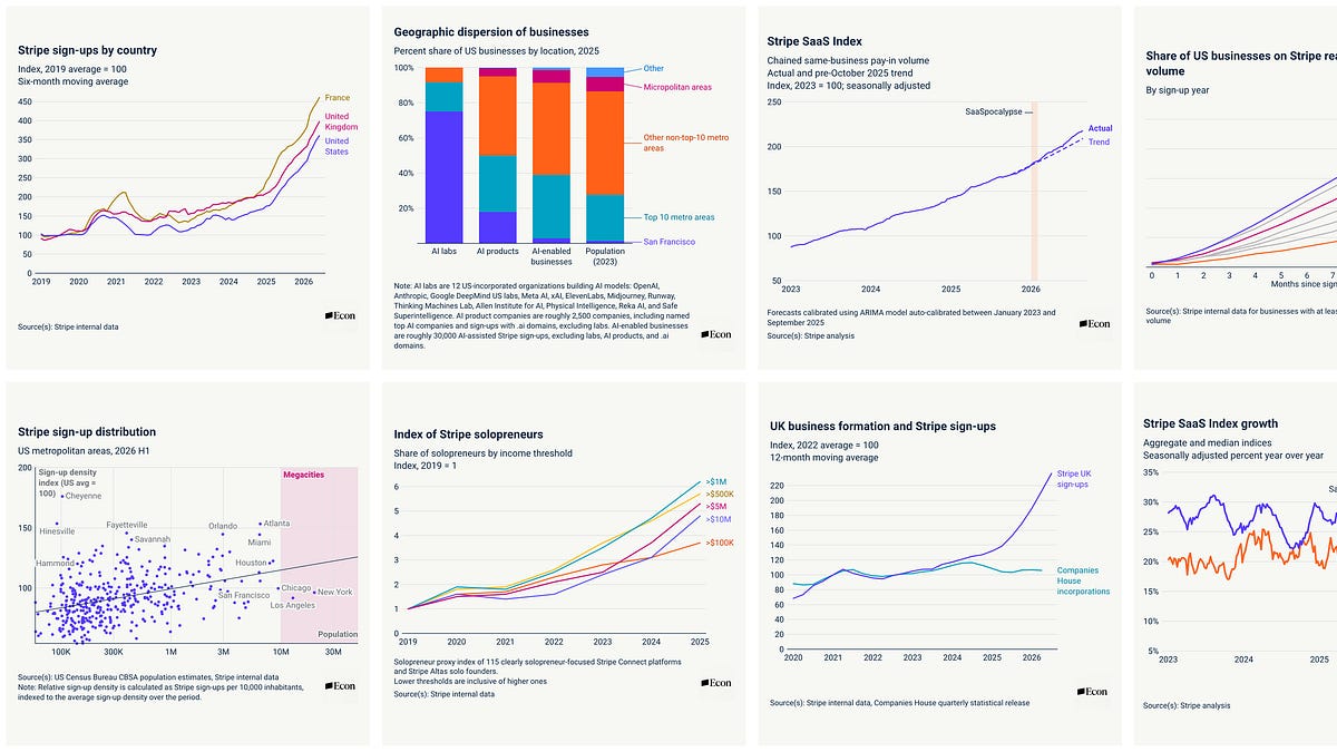
An empirical agenda for AI
Stripe is launching an empirical research agenda to quantify AI's economic impact, leveraging real-time transaction data from 88% of the 'Forbes AI 50'.
Deep dive
- The Data Advantage: Stripe's visibility into payment flows and business formation provides a digital canary for broader economic shifts.
- Productivity Lag: Productivity gains often appear in individual tasks long before they show up in aggregate revenue due to the slowness of market and management adjustment.
- Mimetic Goods: AI may increase the premium on 'human' inputs like judgment, trust, and taste while collapsing the price of routine cognitive labor.
- New Business Formation: Research indicates a surge in solopreneurship, challenging the assumption that AI only benefits massive incumbents.
- Risk Assessment: The agenda seeks to quantify new economic risks, including AI-assisted fraud and the systemic importance of intelligence-as-a-factor-of-production.
Original article
An empirical agenda for AI
Stripe data allows us to see AI’s impact on the economy as it happens.
AI’s economic promise is one familiar to human history: cheaper, more capable tools that raise productivity and prosperity. Even if we assume that AI eventually delivers, much remains unsettled about how, when, and to whom the gains will spread.
Most outside commentary so far has focused on first-order questions, such as AI adoption or token spend, or on the most immediate anxieties around AI, such as automation and job displacement. Those who focus on the long run often do so with either vague promises of a hyperabundant future or predictions of imminent doom. In either case, there are scant details on the path to reach it.
History suggests that many of the most confident predictions about technology are falsified and what gets the most immediate attention is rarely the most consequential. The electrification of America in the early 1920s brought predictions of mass unemployment of factory workers, but not only did US factory employment not fall, it continued rising for more than 50 years, and subsequently declined for reasons largely unrelated to automation. Meanwhile, predictions about the IT revolution boosting aggregate productivity did eventually become true, but only after decades of IT investment and some puzzlement—most famously from Robert Solow—about the lack of obvious effects on the data.
Conversely, the most interesting transformations wrought by general purpose technologies are often second-order and unexpected. Women entering the labor force en masse in the 1960s, for example, was made possible by electrification combined with the complementary innovation of indoor plumbing, as well as other social changes. The internet created entire new job categories that would have been unimaginable to the contemporary commentariat. The majority of employment today is in jobs that did not exist in 1940 and that emerged due to new technologies.
We believe that AI is likely to follow a similar pattern and that we should therefore approach the study of its impact with humility, curiosity, and rigorous empiricism. The answers to how AI will transform society will depend on how businesses reorganize, markets adjust, and workers respond.
But anyone could endeavor to pursue an empirical research agenda related to AI—and many others are—so why do we believe Stripe Economics has anything original to add? The answer is our data. Stripe, via the products it offers and businesses it serves, produces one of the richest real-time datasets on how today’s economy is evolving, including transaction data on payments, sign-up data on business formation, and survey data on business sentiment. To protect the businesses on Stripe, this data cannot be shared publicly, but the insights and analyses this data produces can. This is what Stripe Economics is for.
We’ve already begun using our data in this way to show that there was convergence, not divergence, in spending between high- and low-income areas of the United States. We shed light on what is behind the recent rise in business formation in the US and elsewhere (that is often not being captured in national statistics). We showed how new AI-era businesses are increasingly forming outside major metros and core urban areas. We showed that the AI-driven market turbulence of early 2026 was not reflective of SaaS business reality.
Private data always has some biases. In our case, the primary bias is that Stripe’s user base skews more tech-forward than the economy as a whole. But even this is particularly useful for understanding the current moment. Stripe serves 88% of the Forbes AI 50. We also serve the most tech-forward non-AI businesses, which are digital canaries for how AI is likely to percolate through the economy and affect firms more broadly.
Even with such a privileged starting point, we know that understanding AI’s impact will require data beyond Stripe, approaches beyond economics, and analyses beyond our own. We are sharing our AI research agenda below—and a snapshot of how Stripe data can contribute to answering important questions—to invite others to collaborate with us and contribute. Stripe’s Economics of AI Fellowship already supports early-career researchers studying growth, labor, risk, and market design. We welcome further opportunities for academics, writers, and private-sector researchers to work with us.
Questions we’re thinking about, and how Stripe data can help answer them
The following is a point-in-time snapshot and assumes future access to OpenRouter data (Stripe's acquisition of OpenRouter has not yet closed), as well as the ability to survey Stripe users on topics such as hiring.
- When will aggregate productivity gains materialize?
Economic evidence so far suggests AI is already raising the speed and quality of individual tasks well before those gains appear in revenue, because sales processes, pricing, management, and customer demand adjust more slowly. And if the price of intelligence keeps falling, the net effect on productivity may be pulled in two directions, as lower input costs will drive higher productivity among AI users but might yield lower revenues among AI providers. We expect that AI will eventually move the productivity needle positively, but the interesting story will be the cadence, persistence, and distribution of those gains.
What Stripe data can tell us: the relationship between AI spending and revenue growth, what industries are adopting AI and how intensively
- What will be the unexpected complements of AI?
As Alex Imas has pointed out, AI could increase demand for “mimetic goods” like human relationships, judgment, trust, or taste, even as it lowers the price of routine cognition. Similar to travel agents seeing their jobs decline but value rise in the wake of the internet, AI could lead to a premium on human produced and curated content while AI-driven content becomes cheap and accessible. AI could increase leisure time, but it may alternatively raise expectations of productivity within existing work hours. It’s possible that some of the most transformative changes from AI will come from combining it with complementary innovations, such as domestic robots, drones, or AI-directed wetlabs, that extend its impact from the digital to the physical world.
What Stripe data can tell us: what AI-adjacent sectors are seeing rapid growth, changes in the relative prices of different good and services
- Will AI create new classes of economic risk?
The recent discourse has emphasized the civilizational risk posed by AI, but we’re at least as concerned with the more traditional variety: macroeconomic risks as AI investment ebbs and flows. AI-enabled cybersecurity attacks on critical infrastructure. The use of AI by terrorists and criminal groups. The rise of AI-assisted autonomous weapons. The rise in AI-assisted fraud and scams. The possibility of a future AI-related incident causing meaningful economic and financial harm is a real one, especially as AI becomes more “systemically important.”
What Stripe data can tell us: how spending on AI-related risks (e.g., cyber) is trending, how different sectors of the economy are impacted by new economic risks
- What is the shape of the market for intelligence?
The long-term market structure for intelligence remains unclear. Much of the focus today is on the immediate question of AI lab profitability, but if intelligence becomes a factor of production, then where price and supply of intelligence stabilize will have implications for many parts of the economy. Which jobs are augmented or replaced by AI is at least in part a function of the relative price for humans and machines to execute them. Which new industries emerge depends on how cheaply intelligence can be deployed in pursuit of innovation. Intelligence prices may turn out to have important short- and long-run macroeconomic implications too, in the same way that energy prices do.
What Stripe data can tell us: how token usage and spending are trending, how prices are changing, who is spending more/less on AI, how this relates to various other economic indicators
- How will AI affect labor markets?
Attempts so far to identify AI displacement effects have yielded mixed results, with some showing negative effects and others showing muted or even positive effects, with important differences among different subpopulations, industries, and occupations. And AI may already be impacting employment in unexpected ways. Job postings for software engineers are up over the last two years, despite the fact that AI has “cracked” coding. Digital arts jobs are down since 2022, but live arts jobs are up. AI may also be driving job creation and wage growth in unusual places—for example, among electricians to support data center construction. And it remains difficult to disentangle all of these effects from other economic shocks, such as high interest rates and greater adoption of remote work.
What Stripe data can tell us: (via survey) whether new firms are hiring and in what roles, the relationship between AI spend and headcount, changes in output per employee
- How will AI reshape competition as well as the structure of the firm?
We’ve already seen a surge in new business formation in the age of AI, particularly among solopreneurs. This may prove to be the new equilibrium: more firms that are smaller on average. On the other hand, AI may also mitigate friction that allows companies to become big in the first place. For example, benefits from proprietary models or increased costs of doing business due to new classes of risk (e.g., cybersecurity) could increase returns to scale.
What Stripe data can tell us: how many new firms are forming and where, what sectors they are in, how fast they are growing, how concentrated industries are
- How will agents change broader market dynamics?
Agents go well beyond a simple algorithm and can compare, negotiate, and execute transactions on behalf of humans. This may improve price discovery, reduce transaction costs, and generally increase the efficiency of a wide range of markets. But agents could also be used as rent seekers: looking for inefficiencies and regulations to arbitrage. Sellers will also bring their agents to bear in negotiations, making it hard to predict the net effect on both prices and consumer or producer surplus. And consumer acceptance of a parallel agentic economy is uncertain and will likely be downstream of overall AI adoption.
What Stripe data can tell us: who is using agents to spend, what agents are spending on, how prices change when agents are involved
100+ reactions to 100+ solutions
Prominent mathematicians are expressing significant skepticism following OpenAI's recent claims regarding the mathematical reasoning capabilities of their latest models.
Decoder
- Formal Proof: A verifiable sequence of logical steps leading to a mathematical conclusion, often written in languages like Lean or Coq to ensure machine-checked correctness.
Original article
This post presents a snapshot of the mathematical community's gut feelings regarding OpenAI's announcement on October 6.

The CNCF is graduating projects faster than ever. AI agents are helping with the due diligence
The CNCF is using AI agents to accelerate its project graduation process, citing the need for faster due diligence as AI adoption surges.
Original article
Full article content is not available for inline reading.
_.png)
What is Interactive Application Security Testing (IAST)?
Interactive Application Security Testing (IAST) instruments running applications to find vulnerabilities with high accuracy, but it struggles to scale across polyglot microservices.
Deep dive
- How it works: Uses taint analysis to track input as it moves through the application logic to a sensitive sink (e.g., database query).
- Vs. SAST: IAST is more precise because it sees runtime behavior.
- Vs. DAST: IAST sees inside the app; DAST only sees input/output.
- Trade-offs: Requires language-specific agents, adds runtime overhead, and scales poorly in microservice architectures with diverse tech stacks.
Decoder
- IAST (Interactive Application Security Testing): A security testing method that monitors application behavior from the inside during runtime.
- Taint Analysis: A technique for tracking the flow of untrusted "tainted" data from input to a potential vulnerability sink.
Original article
What is Interactive Application Security Testing (IAST)?
Interactive Application Security Testing (IAST) is a method for finding security vulnerabilities in an application while it's running, by instrumenting the code and observing how it behaves during normal use or testing. Unlike tools that scan code at rest or attack an application from the outside, IAST watches data move through the application in real time. This article explains how IAST works, how it compares to other testing methods, and where it fits in a modern application security program.
What does IAST stand for and what does it do?
IAST stands for Interactive Application Security Testing. It's a category of application security testing (AST) tool that uses instrumentation - small pieces of monitoring code inserted into an application - to observe what happens as the application runs.
Instead of guessing whether a vulnerability exists by analyzing source code or sending external attack traffic, IAST watches real data flows: what comes in through user input, how it moves through application logic, and what the application does with it (like whether it ends up in a database query or gets written to a log unsanitized). This lets IAST confirm vulnerabilities like SQL injection, cross-site scripting (XSS), or insecure deserialization with fewer false positives than some other methods, because it's observing actual behavior rather than inferring risk from patterns.
IAST typically runs during functional testing, QA cycles, or in staging environments - anywhere the application is being actively exercised by a user, automated test suite, or QA team.
How IAST Works
IAST tools deploy an agent inside the application's runtime environment. This agent hooks into the application server, framework, or language runtime (common targets include Java, .NET, Node.js, and Python environments) and monitors specific events as they happen.
The typical workflow looks like this:
- An agent is installed alongside the application, usually in a test or staging environment
- The application runs normally - through manual QA, automated functional tests, or regular usage
- The agent tracks data as it flows through the application, tagging inputs and following them through method calls, database queries, and outputs (a technique often called taint tracking or taint analysis)
- When tainted data reaches a point where it could cause harm without proper handling - like an unsanitized input reaching a SQL query - the agent flags it as a vulnerability
- Findings are reported with the specific code path and line number involved, since the agent has visibility into the actual execution
Because IAST observes real execution paths, it generally doesn't require a separate attack simulation step the way dynamic application security testing (DAST) does. It piggybacks on testing that's already happening.
IAST vs. SAST vs. DAST vs. SCA: What's the Difference?
Security teams often confuse IAST with SAST, DAST, and SCA, since all four aim to find vulnerabilities before they reach production. Here's how they differ, in the order they typically show up across the SDLC.
Static Application Security Testing (SAST)
SAST analyzes source code, bytecode, or binaries without running the application. It's useful early in development because it can flag issues before code is even compiled or deployed, but it tends to produce more false positives since it can't see how the code actually behaves at runtime.
Software Composition Analysis (SCA)
SCA scans an application's dependencies - open source libraries and third-party packages - to identify known vulnerabilities (typically matched against CVE databases) and license compliance issues. It doesn't analyze custom code or runtime behavior at all; it's focused entirely on what's in the software bill of materials. SCA is fast and easy to run early and often, but it flags a vulnerable library version regardless of whether the vulnerable code path is actually reachable or used by the application.
Dynamic Application Security Testing (DAST)
DAST tests a running application from the outside, sending crafted requests (similar to what an attacker might send) and observing the responses. It doesn't need access to source code, which makes it useful for testing third-party or black-box applications, but it can't see what's happening inside the application, so it may miss issues or struggle to pinpoint the exact vulnerable code.
Interactive Application Security Testing (IAST)
IAST sits closer to DAST and SAST in what it observes: it needs the application to be running (like DAST) but has visibility into the code and internal data flows (like SAST). This combination often results in fewer false positives than SAST and more precise, code-level findings than DAST.
That precision comes with real trade-offs. IAST requires deploying an agent inside the application's runtime, which is a more invasive setup than SAST or SCA (neither of which touches a running system) and typically adds some performance overhead. In a microservices architecture, where a single system might span dozens or hundreds of services written in different languages and frameworks, rolling out and maintaining IAST agents consistently can become a significant operational lift - especially if agent support varies by language. IAST also runs later in the SDLC than SAST or SCA, since it depends on a built, deployed, running application, which means issues surface further along in development than they would with static or dependency-based methods.
Most mature AppSec programs don't choose just one. They layer these methods - SAST and SCA early in development, DAST and IAST once the application is running - to cover different blind spots.
Benefits of IAST
Lower false positive rates. Because IAST confirms vulnerabilities using real data flows rather than pattern matching or simulated attacks, findings tend to be more accurate and actionable.
Precise findings. IAST reports typically include the exact line of code and execution path involved, which speeds up remediation for developers.
Works within existing testing cycles. IAST runs alongside functional and QA testing rather than requiring a dedicated security testing phase, which can reduce the burden on security teams and fit more naturally into CI/CD pipelines.
Runtime context. IAST sees how third-party libraries and frameworks are actually used within the application, not just whether a vulnerable version is present - which helps prioritize which issues genuinely need attention.
Limitations of IAST
IAST isn't a complete replacement for other testing types, and it's worth understanding its limits.
- Requires agent instrumentation. Unlike SAST or SCA, IAST needs an agent installed inside the application's runtime. This is a more invasive setup, requires ongoing maintenance as the application and runtime evolve, and adds a layer of operational complexity that agentless methods don't have.
- Performance overhead. Instrumentation adds some runtime overhead, which is usually acceptable in test environments but is rarely used in production for that reason.
- Difficult to scale across microservices. In architectures with many services written in different languages and frameworks, deploying and maintaining IAST agents consistently across the whole estate can be a significant operational burden - particularly if agent support isn't uniform across every language in use.
- Language and framework support varies. Instrumentation agents need to support the specific runtime in use, so IAST tooling may not cover every stack in a diverse environment.
- Finds issues later in the SDLC. Because IAST depends on a running application, it can't catch issues as early as SAST or SCA, both of which can run before the application is even built.
- Coverage depends on test coverage. IAST can only find vulnerabilities in code paths that are actually exercised during testing. If a feature isn't tested, IAST won't see it.
- Requires a running application. IAST can't be used as early in the development lifecycle as SAST or SCA, since there's no application to instrument yet.
Where IAST fits in the SDLC
IAST is best positioned in the testing and QA stages of the software development lifecycle (SDLC), after code is built and deployed to a test or staging environment, but before it reaches production. That timing is the trade-off for its precision: teams get more accurate, code-level findings, but later in the process than they would from SAST or SCA.
Because it depends on the application actually running and being exercised, it works well when paired with automated functional or regression test suites - the more thorough the test coverage, the more thorough the security coverage IAST can provide. Some organizations also run IAST in pre-production environments that closely mirror production traffic patterns.
Practical checklist: is IAST right for your team?
Consider IAST if:
- Your team already has solid automated test coverage (functional, regression, or QA)
- You're seeing a high false-positive rate from SAST or DAST tools that's slowing down remediation
- You need precise, code-level findings for faster developer fix times
- Your applications run on languages/frameworks with strong IAST agent support (Java and .NET have historically had the broadest support - verify current coverage for your stack with your vendor)
- Your architecture is simple enough, or your team has enough platform maturity, to deploy and maintain agents consistently
IAST may be less of a priority if:
- Your test coverage is thin or inconsistent, since IAST's effectiveness is capped by what's actually exercised
- You're testing early-stage code that hasn't reached a running environment yet - SAST or SCA are a better fit there
- You need to assess third-party or black-box applications without runtime instrumentation access - DAST is typically the better tool
- You run a large, polyglot microservices environment and aren't ready for the operational overhead of deploying and maintaining agents across many services
Getting Started with IAST
IAST works best as one layer in a broader application security strategy, not a standalone solution. Pairing it with SAST and SCA for early development feedback and DAST for external-facing risk gives security teams coverage across the entire SDLC, while going in aware of the operational cost that comes with agent-based testing.
If you're evaluating how IAST fits into your existing pipeline, talk to our team about integrating application security testing directly into your CI/CD workflow.

Monitor warehouse data quality beyond pipeline health
Successful pipeline runs do not equal data quality; teams must move beyond job monitoring to implement table, column, and custom SQL checks.
Decoder
- Data Observability: The process of monitoring the health and quality of data pipelines and datasets through automated checks and alerting.
- Schema Drift: The silent changes that occur when upstream data structures (like column types or names) are modified, potentially breaking downstream pipelines.
Original article
You get a Slack message from the VP of Sales: They have asked an AI agent connected to Snowflake for the past quarter’s revenue and the numbers look wrong. First, you verify the agent’s query and, when that looks fine, check the pipelines that populate the underlying table. All jobs completed, the data is recently refreshed. Then it’s time to check the logs for errors. Nothing. So you start querying the table, comparing row counts across runs, and manually reviewing null rates column by column.
After a day of digging, you realize the table has been loading 22% fewer rows than normal for several days, with three key fields nearly half null. No alerts ever fired. By the time you find out, reports were wrong, and decisions may have been made on bad data. You still need to apply the fix retroactively and identify every downstream service, dashboard, or application that consumed the affected data.
Pipeline and data monitoring solve complementary challenges. A failed or abnormally long-running job can be an indication that downstream data is incomplete or delayed. But a completed job does not prove that the right data reached the table. You need to monitor the data produced and transformed by those jobs as well.
In this post, we will explain why successful jobs don’t guarantee data quality, how to detect problems in data at rest, and how to use pipeline-level context to trace the root causes of data quality issues.
Why doesn’t a successful pipeline run guarantee data quality?
Pipeline-level checks tell you whether a data pipeline completed and whether its execution looked normal. Error-rate monitors alert on exceptions, while duration monitors detect jobs that take longer than expected. Long run times can indicate resource constraints, stuck processes, or delayed data delivery.
These checks are essential for measuring pipeline health, but they do not validate whether the right content landed on the table. A pipeline can finish on time, return no errors, and still produce incomplete or incorrect data.
Both the symptoms and the root cause of a warehouse data quality problem can be silent. Common symptoms include:
- Freshness delays: A table or partition is not updated on schedule.
- Unexpected row count changes: A table contains substantially more or fewer records than its historical baseline.
- Nullness or distribution drift: A column accumulates nulls, loses expected values, or develops a different statistical distribution.
- Duplicate or non-unique records: Fields that should serve as unique record identifiers begin repeating.
Some of the common root causes that can also leave pipeline health signals looking normal are:
- Source or configuration changes: An upstream team changes a source connection or filter. The ingestion job completes, but the table reflects a reduced or altered scope.
- Scheduling or dependency changes: A skipped job, failed dependency, or scheduling update prevents a table from refreshing on schedule, with no obvious infrastructure failure to signal it.
- Transformation changes: A dbt model or other transformation is updated with new filtering, join, or aggregation logic. The model runs without errors but produces fewer rows, duplicate records, or unexpected values.
- Schema drift: A field is renamed or its type changes upstream. Depending on how ingestion and schema evolution are configured, the load can complete while affected columns become null, get dropped, or stop mapping as expected.
In each case, the warehouse table still exists and queries return results, even though the content is wrong. No pipeline-level monitor fires. Only a monitor pointed at the data in the table itself would catch the problem.
How to monitor data quality at rest
Monitoring warehouse data quality starts with tracking the data in each table alongside the jobs that produced it. Pipeline signals show whether processing occurred as expected, and data quality signals show whether the output remains usable and trustworthy.
From there, you need to decide what to measure, how to detect abnormal behavior, and how to expand coverage without creating noise or compute costs.
Track the right data quality signals
You can organize data quality checks into four main categories:
- Table-level checks: Use freshness and row count checks to detect stale tables, missing loads, and significant changes in data volume.
- Column-level checks: Monitor nullness, uniqueness, cardinality, and statistical distributions to detect subtler changes within otherwise healthy-looking tables.
- Schema checks: Detect added, removed, renamed, or type-changed columns instead of relying on null rates or custom rules as indirect indicators of schema drift.
- Custom checks: Express business-specific expectations as SQL queries when built-in metrics cannot represent the rule. For example, you might count failed orders or identify records with values that are inconsistent with business logic.
Together, these checks let you detect both obvious failures, such as a table that has not been refreshed, and less visible changes inside tables that look healthy at a high level.
Choose the detection method
Now that you know what to measure, you need to determine how to identify abnormal data. In practice, selecting the right method can be harder than it sounds.
Anomaly detection learns from historical patterns, including seasonality and trends, making it best suited to metrics that vary over time. Because anomaly monitors require 3 to 7 days of training on historical data before they alert, plan for that window when rolling them out on new tables.
During the training window, consider running threshold monitors in parallel as a temporary backstop, using conservative bounds based on recent history. You can then remove or adjust those monitors once anomaly detection has enough signal to operate reliably.
The model can also improve over time when you provide feedback. On a monitor’s status page, you can adjust the expected bounds by marking it as expected, ignored, or a missed alert. This teaches the model what normal looks like for your data. This is useful because data quality metrics are business-specific.
Threshold detection uses a fixed value and works best when you have a hard business rule. For example, a table must contain more than 10,000 rows, or a field should have a null rate below 5%. Static thresholds are a poor fit for most tables because seasonality and volume growth mean that a threshold set today will require constant manual recalibration to stay relevant.
However, a table may appear seasonal but lack enough history for an anomaly detection model to train with confidence. Other tables have business rules that shift with product changes. For example, the meaning of a failed_orders field might change after a platform migration, making threshold maintenance unavoidable.
As a general rule, prefer anomaly detection unless you can express the requirement as a hard, unchanging limit. Most environments use anomaly detection for variable metrics and thresholds for explicit SLAs and invariants. New tables without enough history may require threshold monitors while anomaly models train.
Scale coverage without scaling noise
Once you know how to scope and configure your monitors, the next challenge is keeping the signal-to-noise ratio manageable as coverage grows.
Start with your most important tables and those with the most downstream dependencies, then expand coverage from there. You can group monitors by schema, table, or a custom dimension such as region, so a single monitor covers multiple tables.
When configuring grouped monitors, choose between a multi-alert or simple-alert strategy. A multi-alert monitor sends a separate notification for each group that breaches, such as one notification per affected table. A simple alert aggregates all breaching groups into a single notification, such as one notification for the entire schema. The right option depends on how your teams own and respond to the affected data.
For business-specific rules that built-in metrics do not cover, use custom SQL monitors. For example, the following query tracks failed-order counts as a quality signal:
SELECT COUNT(*) as failed_orders FROM ANALYTICS_DB.PROD.ORDERS WHERE STATUS = 'FAILED'Continue refining anomaly monitors as your environment changes. Annotate known-good or known-bad periods on the monitor’s status page to help the model learn what normal looks like for that dataset. This is useful after expected events such as migrations, backfills, promotions, or seasonal traffic changes.
Monitoring cost and query latency vary by method. Datadog reads warehouse metadata for metrics such as freshness and row count when the warehouse exposes it. Column metrics and custom SQL require direct queries against the table, which can consume warehouse compute and take time to execute. Factor both in when deciding where to use column-level and custom SQL monitors.
Finally, route alerts both to the team that owns the affected table and the on-call pipeline rotation. Notifications can be sent to Slack and email, as well as Datadog On-Call, PagerDuty, and any other channel configured in your notification settings.
How to investigate data quality issues
Once an alert fires, the main questions are: What caused the problem upstream, and what has it affected downstream? Datadog Data Observability’s lineage views answer both by tracing upstream causes and downstream impact so you can assess the overall blast radius.
Most investigations will follow the same sequence:
- Confirm the affected table, column, and time range.
- Use lineage to identify downstream dashboards, models, and dependent tables.
- Determine whether the problem started at the source, in a streaming layer, or during batch processing.
- Bring in Data Observability, Data Streams Monitoring, warehouse query history, logs, and infrastructure telemetry as appropriate.
- Use Bits AI or an AI assistant connected through the Datadog MCP Server to surface relevant telemetry data, map relationships between signals, and accelerate the investigation.
Where you look next depends on the architecture and what your pipeline telemetry shows.
Investigate problems at the source
Not every data quality alert traces back to your pipeline. If Data Observability and Data Streams Monitoring both look normal—with expected throughput, no job failures, and no unusual run durations—the failure likely originated at the source system before your pipeline ever touched the data.
Common causes include an upstream team changing what a feed exports, a third-party data source experiencing an outage, or a source-side filter quietly reducing the scope of records sent downstream.
In these cases, shift the investigation away from pipeline telemetry. Query the source, compare current export volumes with historical baselines, and loop in the team that owns the upstream feed.
Batch pipelines
For batch pipelines, the key question is whether the job processed less input data than usual or processed the same amount of input but produced less output. Those patterns point to different root causes: a reduced upstream source versus a transformation or filtering issue.
Jobs Monitoring for batch loads surfaces per-job metrics, including input and output data volume, run duration, and failure reasons. For Spark jobs, it also exposes idle executor CPU, shuffle I/O, and disk spill. Use side-by-side run comparison to isolate when a drop begins.
Say a row count monitor fires on a Databricks table. Datadog shows that the job completed, but its input data volume was significantly lower than in previous runs. That points to a reduced upstream data source rather than a job failure. From the run view, you can pivot to correlated infrastructure metrics, logs, and cluster configuration for a deeper investigation.
Snowflake and other warehouse-native batch loads may not have a Spark or orchestrator layer. Datadog can detect the problem at the destination table. Row count, freshness, and null-rate monitors read the table rather than the job, so they catch volume or quality changes regardless of how the data was loaded. From there, use lineage, warehouse query history, and source-side checks to find where the data changed.
Streaming pipelines
For streaming pipelines, the key question from a data quality perspective is whether throughput dropped on a specific topic or partition before the data reached the warehouse. Answering it narrows the investigation to the affected producer path without requiring manual querying.
Data Streams Monitoring provides per-topic throughput and lag visibility, showing where volume dropped before it reached the warehouse.
Let’s say a freshness monitor fires on a warehouse table fed by a streaming ingestion service. Data Streams Monitoring can show where throughput diverged across the stream, narrowing the investigation to the affected producer or consumer path. For example, an incompatible schema change could cause the consumer to reject messages even though the producer continues sending them.
Hybrid architectures
In hybrid architectures, a streaming layer feeds batch jobs before data lands in the warehouse. Run the investigation in sequence. First identify where volume dropped in the streaming layer, then confirm whether the lower volume propagated through the batch outputs and reached the warehouse table.
For example, Data Streams Monitoring might show a throughput drop on the input topic, while Datadog Data Observability confirms that the downstream batch job processed less data than during the previous run. Together, the two signals connect the quality issue in the warehouse to a single upstream cause.
Start monitoring your warehouse data
Monitoring pipeline health alone leaves data quality problems invisible until a stakeholder finds them. A job can complete while producing stale, incomplete, duplicated, or otherwise incorrect data.
Datadog Data Observability provides always-on coverage for data at rest and visibility into batch job runs, helping you catch quality issues before they reach stakeholders or undermine business decisions and investigate their causes. Combined with Data Streams Monitoring, you get a connected view from the downstream symptom back through the pipeline to its source.
How Mirelo AI brought sound design to the IDE with MCP and Kiro powers
Mirelo AI brought generative sound design directly into the IDE by packaging its MCP server as a Kiro power.
Decoder
- MCP (Model Context Protocol): An open standard that allows AI assistants to securely connect to external tools and data sources.
- Power (Kiro): An agentic plugin that bundles MCP configurations with specific AI agent skills for task automation.
Original article
How Mirelo AI brought sound design to the IDE with MCP and Kiro powers
Mirelo AI set out to fix how sound design works in the integrated development environment (IDE). For most developers, sound design has always meant leaving the IDE: opening a browser, digging through stock libraries, and trimming and syncing clips by hand. Sound is the last creative layer most developers reach, and the one they most often get wrong without specialist help. For teams building games, apps, and interactive products, digital audio workstations (DAWs) live outside the development workflow, so most ship with placeholder audio or nothing at all.
Mirelo AI, a Europe-based generative AI lab, builds models that turn a text prompt or a video clip into production-ready sound effects, synced to the picture when video is provided. Feed a video clip to the model and it returns audio matched to the action on screen. Mirelo built a hosted server on the Model Context Protocol (MCP), the open standard that lets AI assistants discover and call external tools. With Mirelo’s hosted MCP server, developers can reach those models from the tools they already use.
In this post, we describe how that MCP server became a power in Kiro, the agentic development environment from AWS. We also cover how Mirelo’s AWS Enterprise Support account team helped bring it to the Kiro powers marketplace. The result: Developers using Kiro can generate sound design from a natural-language prompt without leaving their editor.
Solution overview
With a Kiro power, you get Mirelo’s hosted MCP server bundled with Agent Skills that tell the AI assistant when and how to use it. When a developer’s prompt mentions sound, audio, or effects, Kiro activates the power, connects to Mirelo’s server, and loads its tools into the conversation. The developer describes the sound they want. Kiro calls Mirelo’s models and returns a finished audio file into the project.
The design has three parts:
- Mirelo’s audio models, exposed through their existing HTTP API.
- The hosted MCP server (https://mcp.mirelo.ai/mcp), which wraps that API as callable tools.
- The Kiro power, which bundles the MCP configuration with an Agent Skill and publishes it to the marketplace for one-action install.
The problem: Sound is the last mile of creative development
Visual assets have mature tooling inside IDEs and design systems. Audio does not. A game developer prototyping a level generates textures, writes shaders, and tests physics in the editor. But the moment they need a matching footstep sound, the flow breaks. They open a browser, search a stock library, download candidates, trim them to length, and manually sync timing.
Content creators working with generative video hit the same wall from the other side. AI models now produce visual content in seconds, but each clip ships silent, so adding sound means switching tools, breaking flow, and spending more time on audio than the video itself took to create.
Mirelo’s thesis: Sound generation should live where developers already work, not in a separate application.
From API to agent tool: The Mirelo MCP server
Mirelo already had an API powering their Studio product. The question was how to make those capabilities reachable inside AI-powered development environments without asking developers to write integration code.
MCP answers that. By wrapping their API as an MCP server, Mirelo exposed their full audio generation pipeline to any compatible AI assistant. The Mirelo MCP is hosted and remote: developers add a single URL, authenticate through their browser, and start generating audio from conversation. There’s no local install and no API key to manage.
The server covers the full sound design loop:
- Generate from text: describe a sound effect in natural language and receive a finished audio file.
- Generate from video: pass a video clip and get synced sound effects for every action.
- Extend: lengthen an audio clip that is too short for the scene.
- Inpaint: replace a selected region of a clip while leaving the rest untouched.
A preflight tool estimates credits and runtime before generation runs, which matters when an agent works through a batch of files rather than a single effect.
Comparing direct API access with a Kiro power
Without the power, a developer who wants a sound effect works against the API directly. For anything longer than a short clip, that means the asynchronous path: submit the job, get a job ID back, poll for status, then download the result once it completes.
# 1. Submit the job
JOB=$(curl -s https://api.mirelo.ai/v2/text-to-sfx/v1.6/jobs \
  --request POST \
  --header 'Authorization: Bearer sk-<your-api-key>' \
  --header 'Content-Type: application/json' \
  --data '{
    "prompt": "Heavy rain on a metal roof with distant thunder",
    "duration_ms": 45000,
    "output_format": "mp3"
  }' | jq -r '.job_id')

# 2. Poll until the job leaves the "processing" state
while true; do
  STATUS=$(curl -s "https://api.mirelo.ai/v2/text-to-sfx/v1.6/jobs/$JOB" \
  --header 'Authorization: Bearer sk-<your-api-key>' | jq -r '.status')
  [ "$STATUS" = "succeeded" ] && break
  [ "$STATUS" = "failed" ] && echo "generation failed" && exit 1
  sleep 3
done

# 3. Fetch the result URL and download the clip
curl -s "https://api.mirelo.ai/v2/text-to-sfx/v1.6/jobs/$JOB" \
  --header 'Authorization: Bearer sk-<your-api-key>' \
  | jq -r '.result_urls[0]' \
  | xargs curl -o rain.mp3
This works, but the developer owns every step. They store the API key, choose the sync endpoint for short clips and the async endpoint for longer ones, and call preflight to estimate credits. They also run the poll loop with sensible backoff, handle the failure state, download the result, and retry on transient errors. Each surface, whether a web app, a game editor, or a batch script, reimplements the same glue.
With the power, the developer describes the sound and the agent assembles that same request. Kiro authenticates through browser sign-in and reads the tool schema Mirelo published. It fills in prompt, duration_ms, and output_format from the conversation, runs the preflight tool when the job is large, and waits on the async job when generation runs long. The developer writes:
Generate 45 seconds of heavy rain on a metal roof with distant thunder, as an mp3.
The file is added to the project. The underlying API call is the same. What changes is who assembles and operates it.
| Concern | Direct API | Kiro power/MCP tool call |
|---|---|---|
| Authentication | Store and send Bearer sk-… on every call | Browser sign-in, managed by Kiro |
| Cost check | Call /preflight yourself | Agent calls the preflight tool when the job warrants it |
| Sync compared to async | You choose the endpoint and implement polling | Agent selects based on job size |
| Response handling | Parse result_urls and download | Agent returns the file into the project |
| Reuse across tools | Reimplement the glue per surface | One power, available in any Kiro session |
Why package it as a Kiro power
Mirelo’s MCP server already worked in several AI assistants. With a Kiro power, you get discoverability, so you find the integration while browsing the marketplace, and automatic activation, so there is no URL to paste or configuration to write.
A power bundles an MCP server with Agent Skills, the structured instructions that guide an AI assistant through a specific workflow. The AI assistant learns what tools exist and when to reach for them. Just as important is how a power loads. A traditional MCP setup registers every tool definition upfront. Connecting a handful of servers can burn tens of thousands of tokens, a large share of the context window, before your first prompt. Kiro powers load dynamically instead. Installed powers sit dormant until your conversation mentions relevant keywords, at which point Kiro activates only that power’s tools and skills and deactivates them when you move on. Skills load the same way, on-demand, so the AI assistant pulls in a specific workflow’s instructions only when it’s working on that task. The result is near-zero baseline context cost and a Mirelo integration that surfaces its sound-design tools exactly when they’re needed, without crowding out the rest of your work.
The structure of a power is small. The following layout shows the three files that define it:
example-power/
|-- plugin.json          # Manifest: name, keywords, and metadata
|-- mcp.json             # Remote MCP server configuration
+-- skills/
    +-- sound-design/
        +-- SKILL.md     # Guides the agent through audio workflows
The plugin.json manifest declares the keywords that trigger activation. The mcp.json file points to the provider’s hosted server. The skill teaches the agent the difference between generating a one-shot effect and sound-designing an entire sequence.
The path from idea to marketplace
The Kiro powers connection came from Mirelo’s AWS Enterprise Support account team. The team spotted the fit between Mirelo’s MCP server and the powers marketplace. They built a proof-of-concept power to show how the integration would work and connected Mirelo with the submission process. Mirelo then packaged their official hosted server as the published power.
From the first conversation to a live power took about two weeks, most of it marketplace review. The engineering itself fit into a single afternoon. The impact is easiest to see in the developer’s workflow. Finding a single sound effect that matches the video is slow, manual work. That includes searching a stock library, auditioning candidates, trimming, and syncing. With the power, a single prompt returns a usable, synced clip, replacing a lengthy manual workflow with one step.
What developers can do with it
After the Mirelo power is active, sound design becomes part of the conversation. A developer polishing a web app might ask:
Generate a soft, satisfying click for this submit button. Short, no metallic ring.
On a game prototype, the request could be:
Here’s my gameplay clip. Generate footstep and impact sounds that match the character’s movement.
For a video project that needs a longer bed:
Extend this forest ambience to forty-five seconds so it covers the full scene transition.
And to fix a single moment:
The glass-break sound at 0:03 is too harsh. Inpaint that region with something more subtle, like thin crystal.
Each request calls Mirelo’s models and returns audio ready to use, without the developer leaving the editor.
A distribution channel for AI model companies
For Mirelo, the Kiro powers marketplace is a new kind of distribution. API businesses have historically reached developers through documentation sites, SDKs, and marketing. A power puts the capability inside the tool developers already use. Developers reach it by intent rather than by integration work.
The model fits AI services that augment creative workflows. Developers don’t plan to use a sound API the way they plan to use a database. They need sound the moment they realize their project is silent. A power meets them at that point of intent.
Conclusion
In this post, we described how Mirelo AI turned a hosted MCP server into a Kiro power, and how AWS Enterprise Support helped move it into the marketplace. For developers, sound design is now a prompt away inside Kiro. For AI model companies, the same path turns an existing MCP server into a distribution channel that reaches developers at the point of intent.
To get started:
- Install the Mirelo power from the Kiro powers marketplace.
- Try Mirelo and connect the hosted MCP server to your AI assistant.
- Read the Kiro powers creation guide to package your own MCP server.
- Review the Agent Plugins specification to build portable, vendor-neutral plugins.
ChatGPT can imitate a cartoonist. Now it's signing their name, too
OpenAI's image generator is creating cartoons that include signatures from real-world New Yorker artists, potentially causing deceptive attribution.
Deep dive
- Artists found that ChatGPT can produce images that mimic their unique artistic style and include a synthetic version of their signature.
- The issue highlights the difficulty of enforcing 'style' restrictions when models can generate variations of existing signatures.
- OpenAI has attempted to implement keyword-based filtering, but it is currently ineffective at stopping all instances of signed outputs.
Original article
ChatGPT has generated cartoons containing signatures associated with more than 15 New Yorker contributors, potentially making AI-generated work appear to have been created by real artists. Cartoonists including Brendan Loper and Emily Flake have encountered images bearing recognizable versions of their names despite having no involvement in creating them. OpenAI has introduced warnings for some New Yorker-style requests, but signed outputs have reportedly continued to appear, raising concerns that style imitation can cross into false attribution.
Any Website's Design, as a Prompt for Your AI (Website)
A new Safari extension captures live website design tokens, including color, type, and layout, to feed structured prompts directly into coding agents.
Decoder
- Coding agent: An AI model or tool designed to write, refactor, or debug software code based on natural language or structured prompts.
Original article
A Safari extension for Mac that measures any website's colors, type, spacing, and layout, then hands it to your coding agent as one measured prompt.

Information Architecture Works at Different Scales
Information architecture is not a monolithic practice, but a tiered discipline where constraints change depending on whether you are designing an interaction or organization.
Deep dive
- IA scales are nested: organizations contain platforms, which contain sites, which contain interfaces, which contain interactions.
- Higher-level architectures constrain lower-level ones; decisions made at the platform level dictate the possible taxonomy and metadata available for individual sites.
- Unlike traditional static blueprinting, modern IA functions more like interior design where you must work within the limits of existing platform components and fields.
- Different layers of an architecture move at different speeds, which leads to misalignment over time.
- Comparing IA effectiveness is only valid when comparing architectures at the same scale.
- Design is a continuous oscillation between context and artifact, where understanding the larger environment (e.g., the organization) is necessary to build effective components (e.g., the interface).
Decoder
- Information Architecture (IA): The structural design of shared information environments; the art and science of organizing and labeling websites, intranets, online communities, and software to support usability and findability.
- Taxonomy: A scheme of classification or a hierarchical categorization of content.
- Metadata: Data that describes other data, such as tags or attributes used to classify content within a system.
Original article
Information architecture works at different scales
Key takeaway: To evaluate an information architecture, first identify at what scale it operates. Information architecture generally applies to one of five scales: The organization, The platform, The site, The interface, or The interaction. At each scale, information architecture operates with different constraints. Each scale changes at different rates, and each scale operates within a different design context. Scale gives us a way to classify the type of information architecture, so we know what we can compare. Platform to platform and site to site.
5 years ago, I was called in to help a global energy company migrate from their digital marketing sites from one platform to another.
It was one of those swanky consulting gigs. Posh hotels, exciting restaurants, trips to key cities around the world…
Their current platform had been discontinued and vendor support was due to shut down. They needed to move to a living, supported platform.
So we interviewed stakeholders. We talked to seven, separate lines of business and discovered they didn’t just have a vendor support problem. They had a platform problem. The current platform was slow to update and make changes, so they never tried anything new. The current platform provided only basic analytics, so marketing teams weren’t sure what worked, and it was slow and expensive to launch new sites.
We didn’t just move them to a new platform. We transformed how they went to market with a new, customized digital marketing platform. From the original seven sites, the platform has since launched 100s of websites across 12 different business lines in over 9 languages in countries all over the globe. Time for updates went from weeks to days, so content and campaigns are always up-to-date. Time to launch new content went from months to weeks, and the time to launch new sites went from years to months. In addition, the cost to launch a site went down 66%, organic traffic was up for most business lines by 20% Year over Year, lead generation up as much as 150%, and analytics are built into every component, so the marketing team now has detailed data on how content, personalization, and campaigns perform. Of all the things I’ve ever worked on, this is one of my greatest designs.
And it looks like this.
We delivered a platform. Not a site. We delivered a platform the client could use to build sites. We did some wireframes, but they were conceptual to show what could be done and weren’t used to design individual sites. We created no site taxonomies, did no content audits. We delivered no templates.
But the IA we created gave the client and its vendors the language and mental models they needed to build their sites. Instead of taxonomies, we gave them metadata and classification systems. Instead of templates, we gave them layouts and components, so they could design and build their own pages.
Now, there’s an old mental model floating around that likens IA and other design pursuits to creating blueprints before you build the house.
This was true 15 years ago when there were no platforms or useful, off-the-shelf software for building sites. Nowadays, it’s more like interior design. Someone else has already laid the slab and built the walls. You already have the platform. You come in, hoping it has good bones, and make it somewhere livable.
Nowadays, I.A. is more Fixer Upper than Frank Gehry.
Most times, you don’t design the best taxonomy, you design what the platform will allow. You don’t leverage the metadata you need, you use the fields the platform makes available.
So, sometimes IA works at the platform level,…
and sometimes IA works at the site level. At each level, you do the same kinds of activities with different types of inputs and outputs.
If we continue our fantastic journey, our scale grows narrower because sites are made up of interfaces.
Just like with platforms and sites, to architect good interfaces, we must understand the mental models, their pieces, and how they should be joined.
Just as platforms are places where sites occur, and sites are places where interfaces occur, interfaces are places where interactions occur.
To architect one level, you need to understand the foundation it creates for other scales. For example, to architect the platform for the oil giant, I had to understand what kinds of sites they wanted to build. To understand those sites, I needed to understand the types of interfaces they might want to design. To architect those interfaces, you need to understand the type of interactions they want to enable.
The information architecture at the larger scale constrains the architecture at the smaller scale. As John Culkin wrote:
“We shape our tools and then the tools shape us.”
For the oil giant, I shaped the platform, and then the platform constrained what type of sites could be built.
These constraints ripple across all scales. The sites suggest possible interfaces. Possible interfaces allow possible interactions. The shape of the tool echoes through what the tool helps you build.
You hear the echoes elsewhere as well. One of my favorite quotes comes from architect, Eliel Saarinen:
“Always design a thing by considering it in its next larger context – a chair in a room, a room in a house…”
Because I understood the sites the client needed to build, I was able to design the platform.
As an aside, these two quotes illustrates design’s fundamental tension: context drives the design and the design creates the context.
The oscillation from the room to the chair to the ass that sits there.
As information architects, our work oscillates across different scales.
Understand the site to design the platform you need. Understand the platform, and you can imagine Saarinen’s room. Understand the platform, and you can imagine the organization that uses it.
To design the room, consider the house. Design requires we work at different scales.
Why should we care about working at different scales? Because you’d be hard pressed to compare the information architecture of the oil giant’s platform with the IA of one of its sites. Comparing the IA of one site to another is easy.
The pre-requisite to a disciplined, systematic study of information architecture is to recognize scale changes IA in significant ways, and if we want to compare IAs, we must do so within the scale. Platform to platform. Site to site.
- A platform can have many sites.
- A site can have many interfaces.
- An interface can have many interactions.
- An organization can have many platforms.
- A culture can have many organizations.
These scales assimilate the way many of our colleagues slice the world and even echo in the work of influential thinkers like Gibson.
The information architecture at each scale is affected by different forces.
One of those forces is the pace of change.
You’ve probably seen a diagram similar to this showing each level as a different pace layer. This is based on a similar diagram about buildings from Stewart Brand. That is: each layer moves at a different pace. The information architecture at each scale changes at a different pace.
In this case, the outside moves faster than the inside. You might think this works like a bike tire where the entire wheel moves in synch and everything stays aligned.
But Brand’s observation was not only that each layer moved at a different pace, but that these different paces sheared the layers away from one another. So the rotation is really more like a solar system where the planets all move at different speeds.
Although the needs and capabilities at each scale may align when you design them, the different speeds mean each layer immediately begins to shear out of alignment with the others.
Shearing means you are only aligned once, and the more and more out of alignment, the more likely the layers will shear off from one another. The information architecture at each level always exists at a different point in time. You can’t compare one scale to another because the context at the time of design and the context at time of use are always different.
The chair changes faster than the room, the room faster than the house. Sooner or later, the house, room, or chair aren’t what you need anymore.
So, to evaluate an information architecture, first identify at what scale it operates.
Information architecture generally applies to one of five scales:
- The organization
- The platform
- The site
- The interface
- The interaction
At each scale, information architecture operates with different constraints. Each scale changes at different rates, and each scale operates within a different design context.
Scale gives us a way to classify the type of information architecture, so we know what we can compare. Platform to platform and site to site.
Xbox Expands Movie, TV Ambitions With New Division
Microsoft is transitioning Xbox from a gaming hardware business to a broader entertainment studio model spanning film, TV, and theme parks.
Original article
Xbox's entertainment division will grow Xbox's footprint in film, TV, products, events, and theme parks.
Imperfection
Developer Mamuso's site redesign demonstrates how 'pointless' imperfections, like fake game cartridges and microphone-sensitive animations, can make personal projects more engaging.
Deep dive
- Uses View Transitions API to create fluid, paper-like movements for image galleries.
- Implements custom shaders to mimic physical material properties like creased paper and glossy plastic.
- Uses Web Audio API to detect microphone input, allowing users to 'blow' on elements to trigger animations.
- Focuses on 'non-optimized' interactions to build personality, contrasting with typical performance-obsessed enterprise web development.
Decoder
- View Transitions API: A browser native feature that enables smooth, animated transitions between different states or pages without requiring complex external animation libraries.
- Shader: A small program written in a language like GLSL that instructs the GPU how to render lighting, texture, and surface appearance for graphical elements.
Original article
A personal website redesign became an excuse to explore deliberately playful details, including fake game cartridges for past jobs, draggable photo prints, paper-like shaders, animated labels, unusual links, and dynamically generated social cards. Many of these touches serve little practical purpose, but that lack of optimization is precisely what makes the process enjoyable and gives the site its personality. Personal projects can create space for experimentation that professional work often removes, making unnecessary details, imperfection, and prolonged tinkering valuable in themselves.
Energy Icons — energy transition icons (Website)
This open-source library provides over 1,200 specialized icons for energy, climate, and decarbonization projects.
Original article
Energy Icons is an open-source library of more than 1,200 icons for energy and climate products, covering areas such as renewables, electricity, transportation, buildings, and decarbonization in two optical sizes and two weights.
Create Physical Products (Website)
Autonomyware claims to use autonomous systems to engineer physical products from conceptual ideas.
Original article
Create physical products with Autonomyware: everyday objects, complex systems, sculpts, and toys, engineered autonomously from your idea.
Mother Design exercises restraint with new M&S pack system
Mother Design overhauled M&S packaging by replacing fragmented sub-brands with a unified, grid-based information design system.
Original article
Mother Design has created a restrained packaging system for thousands of M&S Home and Lingerie products by removing competing sub-brands and hierarchies and looking to classic information design rather than other retailers for inspiration. The system standardizes MS London typography, introduces a geometric numeral set called MS London Geo, and uses grids, consistent hierarchy, restrained colors, and color-coded sizing to make complex product information easier to navigate. Packaging materials, photography, and tone adapt between Home and Lingerie while maintaining a shared structure designed to strengthen the M&S master brand and scale into additional categories.

Street Artist Turns Graffiti Letters into Neon Portals Where Typography, Architecture, and Science Fiction Collide
Artist Javier Demsky transforms graffiti letterforms into complex, science-fiction-inspired geometric sculptures.
Original article
Spanish artist Javier Demsky, who started in graffiti in the early 1990s, bends the letters of his name into luminous structures blending typography, architecture, and science fiction.